Loading component...
At a glance
Many jobs require the use of Excel in some capacity. This is true of accounting and finance roles, where Excel is essential, and mastery of the software is an important skill.
While many graduates have basic Excel skills at the start of their career, these tips will help them to develop their skills to be more productive and confident in the short term – and more employable in the long term.
Getting started
The major areas to focus on when starting out using Excel are listed below, with links to articles on some of these topics to enable ongoing learning. Some bonus topics are also included.
Sharing useful Excel tips and shortcuts around the office is a great idea.
Structure
Each individual Excel file is called a workbook. When building Excel files, it is important to split the file into separate sheets or tabs.
Splitting the file in this way makes formatting and formulas easier to both create and maintain.
Sheets can also be colour coded, and there may be multiple sheets of each type within a single file. Common sheet types are listed alphabetically in the table below.
| Sheet type | Usage |
|---|---|
| Assumptions | Lists underlying assumptions behind the file |
| Dashboard | Contains data summaries using data visualisations, including charts and icons |
| Data | Contains the data that forms the basis of both reports and dashboards |
| Documentation | Describes how the file works |
| Inputs | Areas to enter data manually |
| Instructions | Explains why and how to use the file |
| Lists and tables | Contains the lists and lookup tables used in the file |
| Report | Contains final reports |
| Validations | Used to check that everything that should balance does balance |
| Workings | Areas to enter interim calculations |
Formula basics
The basic building block of a spreadsheet is called a cell. A cell can contain numbers, text and dates, as well as underlying formulas.
A group of cells is called a range. Most formulas work with both cells and ranges.
A cell is referred to by its column number, then its row number, such as A1 or C100.
A range is referred to by its top-left cell, then its bottom-right cell, separated by a colon, such as A1:C100 or B7:B54.

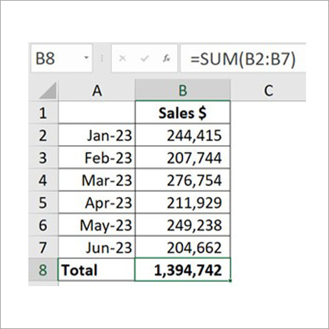
Formulas can perform all the standard mathematical operations. Functions, such as SUM (See Figure 1), perform specialised calculations (see Function basics).
All formulas must start with the = sign. A little-known hack is that you can start a formula with the + sign. When you press Enter, Excel will insert the = sign at the start of the formula.

A full-size keyboard includes both a large + sign and a large Enter key on the numeric keypad on the far right (see Figure 2).
The large + sign is easier to access than the = sign, which is tucked away in the middle of the keyboard. The numeric keypad on the right is also useful because it includes the most common formula operators, and it uses the calculator number layout.
Cell references
When referring to cells and ranges, it is important to understand the use of $ signs.
There are three types of cell references – relative, absolute or fixed, and mixed.
- A relative reference is the standard reference, e.g. A1. A relative reference can vary when formulas are copied. Sometimes this is not what you need, so you must use one of the other reference types.
- An absolute or fixed reference, e.g. $A$1, will never change, no matter where it is copied.
- A mixed reference, e.g. $A1 or $A2, includes a $ sign, which stops the reference it precedes changing when the formula is copied to other cells.
A combination of each reference type can help to create a single formula that can be copied across and down to fill a range.

Pressing on the F4 function key (see Figure 3) when editing in the Formula Bar will toggle between the reference types, in the order shown.
A1 [F4] → $A$1 [F4] → A$1 [F4] → $A1 [F4] → A1
This sequence is consistent, so you quickly learn how many presses are required to get the reference you need.
First rule of Excel formulas
Never enter a value into a formula if that value could change. Values that can change should be entered in a labelled input cell instead.
That input cell is what should be referenced in the formula, rather than its value. This means that if a value must change, only a single cell need be changed – rather than every formula that used that value.
Functions basics
Excel has functions that perform specific calculations. The most-used function is SUM, which adds up the values in a range. Knowing how to use SUM will aid in the use of AVERAGE, COUNT, COUNTA, MIN and MAX, which all use the same function layout (called syntax) as SUM.
Excel has hundreds of functions, but you only need to master about 20 to 30 to be an advanced user.
The following functions, listed alphabetically in the table, are useful for starting out in Excel.
| Function | Description |
|---|---|
| AVERAGE | Returns the average from a range of numbers |
| COUNT | Counts how many numbers and dates are in a range |
| COUNTA | Counts how many entries are in a range |
| COUNTIFS | COUNT, but based on specified conditions |
| EDATE | Adds months to a date |
| EOMONTH | Returns the last day of a month |
| FILTER and SORT | Automate extracting filtered and sorted entries from tables – new functions only available with Microsoft Office 365 subscription |
| IF, IFS | Builds decision-making into a file |
| IFERROR | Handles all formula errors, except the new #SPILL! error |
| MIN | Returns the minimum from a range of numbers |
| MAX | Returns the maximum from a range of numbers |
| ROUND | Rounds numbers to specified decimal places |
| SEQUENCE | Provides a list of sequential numbers, useful for monthly reporting, budgets, and forecasts – new function only available with Microsoft 365 subscription |
| SUBTOTAL | Used to create subtotals and grand totals in lists – works well with filtered lists and can add up just the visible (filtered) cells only |
| SUM | Adds up multiple ranges in a single function, and can also perform a 3-D SUM through multiple sheets |
| SUMIFS | SUM, but based on specified conditions |
| TEXT | Formats dates and numbers into text so they can be used with other text – also used to create dynamic report headings |
| TEXTJOIN | Joins ranges of text together |
| TODAY | Returns today’s date |
| UNIQUE | Extracts a unique list of entries from a list – new function only available with Microsoft 365 subscription |
| XLOOKUP | Flexible, robust lookup function to extract entries from a table, replaces VLOOKUP and HLOOKUP – new function only available with Microsoft 365 subscription |
| YEAR, MONTH and DAY | Return their name as a number from a date |
Formatting
How a spreadsheet is formatted can make a huge difference to how easily it can be used and understood. Using the right number format makes reading numbers easier.
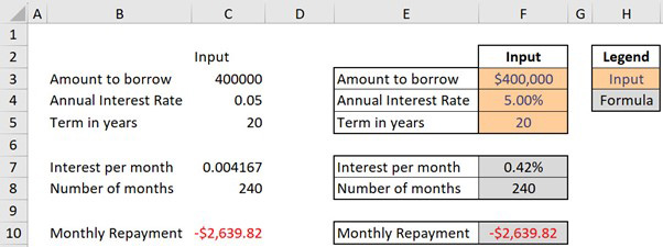
In Figure 4, the entries in columns B and C have no formats. The same entries in columns E and F have been formatted.

Formatting suggestions
- Be consistent with formats throughout the file. For example, use a consistent cell fill colour for all input cells.
- Use Styles from the Home ribbon. These make it easier to apply consistent formats.
- Use colour sparingly and for effect.
- Be aware of colour blindness. Men are most affected by colour blindness and it mainly affects red/green recognition.
- Consider using pastel colours rather than bright colours.
- The comma format is useful for large numbers, such as 1,234,567 instead of 1234567.
- Avoid using the $ format for all the numbers in a report – instead, place the $ sign in the column heading.
Conditional formats
Conditional Formatting is a special feature within Excel, which allows users to vary the format of the cell based on the value in the cell. Conditional Formatting is accessible on the Home ribbon.
This feature can automate exception reporting and can be used for reports and dashboards.

Keep colour-blindness in mind when creating conditional formats. Red-green colour blindness is the most common, so the typical traffic light report (green is good, red is bad) can be problematic.
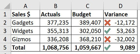
Consider using coloured icons like ticks and crosses (see Figure 5), which are available with conditional formats.
Charts
In Excel, a graph is called a chart. The ability to create data visualisations is an important skill for accountants and finance professionals. Using charts to summarise large datasets can provide many insights that are hard to identify in standard reports.
- Use colour for effect – but keep it simple.
- Start with column, bar and line charts.
- Use pie charts sparingly.
- Avoid all 3D charts.
Printing
The process to print a document in Excel differs from printing in Outlook, Word and PowerPoint.
When you hit the print icon in Excel, the default setting is to print every cell that has an entry on the sheet. That can require a lot of paper!
To restrict Excel printing, set the print area for each sheet. This is a good habit to adopt. The print area icon setting is on the Page Layout ribbon tab (see Figure 6).

Another issue when printing large reports is how to display the row and column headings across multiple pages. The row and column headings need to be repeated on each page. In Excel, these are called Titles and you can set them on the Page Layout ribbon.
Always check the print view before clicking print to avoid accidentally printing reams of paper. Click the File tab and then click the Print option on the left to see a preview of the printed pages. The total number of pages is listed at the bottom of the screen.
Shortcuts
As you develop your Excel skills you will find there are lots of shortcut techniques. I covered many of them in the June Excel Tips article. These can save you a lot of time and effort.
Bonus topics
The following topics are more advanced but important in accounting and finance.
Format as Table
The Format as Table feature instructs Excel to treat a table like a small database. The main advantage is that the table automatically expands to include new rows and new columns. Formulas are also automatically copied down the columns.
PivotTables
PivotTables are used to summarise large datasets in the click and drag of a mouse button. No formulas required, and the reports are easily converted into a PivotChart.
Power Query
The Power Query feature has changed how data is imported into Excel. It automates the process and allows users to fix the data as it is imported.
Real-world data sources often have problems that need to be resolved before the data can be used in reports and formulas. Power Query can automate the correcting the data in a process called “data cleansing”, so that when you refresh the data the latest data is ready to use.
Dynamic arrays
This new calculation engine in Excel allows for more dynamic, flexible formulas that automatically expand based on the data or instructions given.

