Loading component...
At a glance
PivotTables are one of Excel’s most powerful features. They have the ability to summarise huge data sets into a table-based report with a few mouse clicks.
PivotTables have a drag-and-drop interface that allows you to design and change your reports using only the mouse, without writing a single formula.
Even though you don’t need any formulas to create a PivotTable, there is a built-in feature that allows you to perform basic calculations within the PivotTable.
I have seen PivotTable reports with columns added by the user on the right-hand side of the report that perform other calculations based on the values within the PivotTable.
In many cases these additional calculations could be performed within the PivotTable itself.
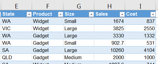
As a simple example examine the data extract in Figure 1.
I’ve used the Format as Table icon on the Home ribbon on this data table. We covered this feature in the August 2018 edition of INTHEBLACK. I highly recommend that you use
Format as Table on any data table that you use with PivotTables. The table will automatically expand as data is added to it. When you refresh the PivotTable any extra data is automatically included in the PivotTable.
Refreshing a PivotTable
When a PivotTable is created all the data is copied into the computer’s RAM, into what is called the PivotCache. This is where the data comes from to create the PivotTable. If you change the underlying data nothing changes in the PivotTable report until you refresh the PivotTable. Refreshing the PivotTable report updates the PivotCache with the latest data, which then updates the report.
Figure 1 includes Sales and Cost. We need the margin and the margin percentage. We could add another column into the data table for the margin, but not the margin percentage. We can calculate the margin and margin percentage within the PivotTable by using what is called a Calculated Field.
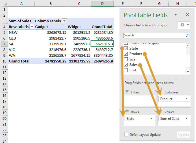
Figure 2 shows a simple PivotTable report (left) and the PivotTable Field List (right).
To create a PivotTable click a cell inside the formatted table, click the Insert ribbon tab, then click the PivotTable icon (far left) and click OK. Drag the field names to the various sections of the PivotTable, see the arrows in Figure 2. When dealing with PivotTables a field is a column of data.
The option we require is called a Calculated Field.
Creating a Calculated Field
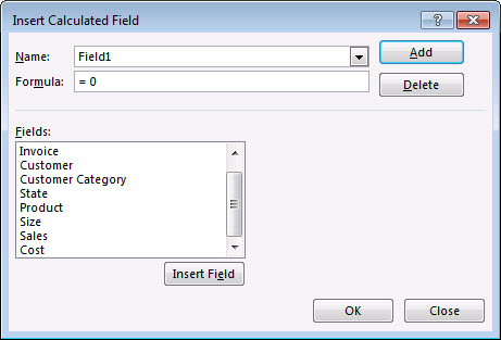
Click any cell within the PivotTable report, then click the Analyze ribbon tab and click the Fields, Items, & Sets icon dropdown and select Calculated Field. (In Excel 2010 the tab is called Options). The dialog in Figure 3 will display.
The name you create can include spaces and special characters like the percentage sign.
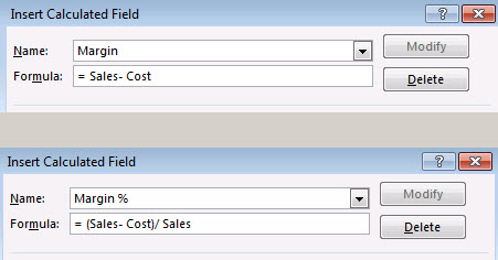
In the Formula box you create formulas by double-clicking the field names listed in the Fields section below. You can also use basic arithmetic operators like + - / * to do calculations. In our case, we need to subtract the cost from the sales field to arrive at the margin. We can click the Add button, then create another Calculated Field for the margin percentage. Clicking the OK button will add both fields to the PivotTable. Figure 4 shows the completed formulas for both Calculated Fields.
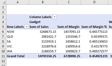
Figure 5 shows an extract of the revised PivotTable report, which now includes the two Calculated Fields. The Margin % could also have been created using the formula =Margin/Sales. Once you have created a Calculated Field you can use it just like a normal field name.
There is one problem with this technique when used for percentages: the heading in the report includes the text “Sum of”. This is not accurate in terms of the calculation being performed.
A little-known technique with PivotTables is that you can rename the headings in a PivotTable report. In our case, we could amend cell D5 in Figure 5 and delete the words “Sum of” and add a space to the end of Margin %. When amending PivotTable column names, you can’t use an existing field name or a Calculated Field name. By adding a space to the end of the heading name, you differentiate it from the field name and it will be accepted.
You will likely want to change the formats on the columns, especially the percentage column. Unfortunately, no formats are applied to values in a PivotTable. The best way to format a column or columns is to right-click a cell(s) in the column(s), then choose Number Format and make the necessary changes. In general, don’t use the Format Cells option on a PivotTable report as it requires you to select a range. With the Number Format option you can select a single cell in a column and the new format will be applied to the whole column, even if it expands in future changes to the report.
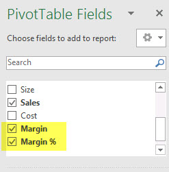
When you create a Calculated Field it is added to the PivotCache and it will appear in the Field List of other PivotTable reports that use the same PivotCache. See Figure 6, which shows the two new Calculated Fields.
Double-click trick
This is a technique that many people find out by accident. If you want to see the underlying data that makes up a specific cell in a PivotTable report, simply double-click that cell. Excel will create a new sheet with all the data records that make up that cell. This is a separate sheet to the source data and is a copy of the records involved.
The companion video and Excel file will go into more detail to demonstrate these techniques.
Neale Blackwood CPA runs A4 Accounting, providing Excel training, webinars and consulting services to organisations around Australia. Questions can be sent to [email protected]

