Excel tips: how to use 'Format as Table' icon as a database

The Format as Table icon on the Home ribbon tab was added in Excel 2007. Unfortunately, most people think it is a formatting feature. Rather, it is a database option. By using the Format as Table icon you instruct Excel to treat a table like a basic database.

Formatted tables have many advantages, such as:

1. The table range automatically expands (including the format) when you add new rows or columns to the table.
2. Filter icons are automatically added to the header row.
3. The headers are always visible as you scroll down the table.
4. Structured references are automatically created; these are like range names and will be explained later.
5. Using a formatted table as a data source for a PivotTable means that any extra rows or columns are automatically included when the PivotTable is refreshed.
6. Formulas are automatically copied down columns. This occurs when creating or editing formulas and when new rows are added.
7. There are extra options on the right-click menu and the Insert and Delete options work well with a formatted table.
8. Some keyboard shortcuts work slightly differently (in a positive way) when used inside formatted tables.
9. Formatted tables work seamlessly with Power Query and PowerPivot. In Excel 2013 and later versions they are required when using the Relationships icon in the Data ribbon.

Some of the disadvantages of formatted tables are:

1. Applying sheet protection can affect some functionality of formatted tables.
2. Excel’s Sharing feature (Review tab) is affected by formatted tables.
3. You can’t use the automated subtotal feature within a formatted table.
4. Sometimes a formatted table will limit the ability to copy a sheet.
5. Copying structured references across with the fill handle doesn’t always provide the desired result, which will be further explained.

Example

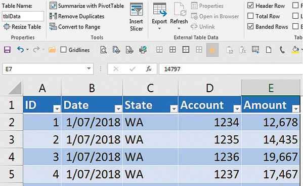
I have used the Format as Table icon on the table in Figure 1.

Excel automatically names each table with a unique generic name; e.g. Table1, Table2, etc. You can rename the table in the Design tab that opens when you click in the table. I have renamed the table to tblData – see top left of Figure 1. My naming convention uses a prefix of tbl to differentiate table names from range names.

Structured references

Table names can be used in formulas. In Figure 3 I have created a VLOOKUP formula in cell H2 demonstrating the use of the table name. Column I displays the formulas in column H. The table name tblData acts like a fixed reference and won’t change as the formula is copied across or down.

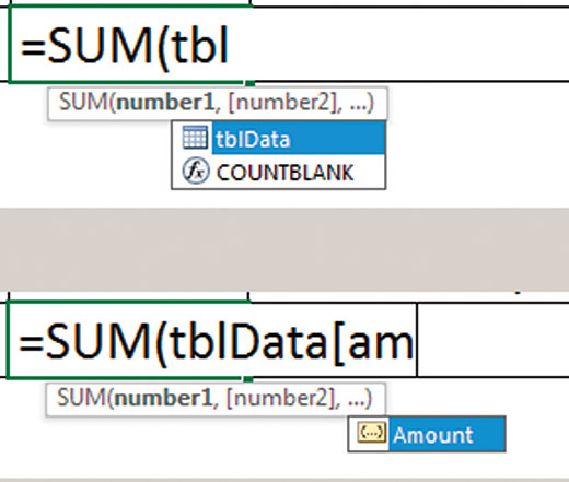
As well as the table name, each column in the table can be referenced using what are called “structured references”. The formulas in cells h2 and H4 in Figure 3 demonstrate how to refer to the columns in a formatted table. These references automatically expand as data is added to the table. Column names are entered between square brackets following the table name. You don’t need to type all the characters in the names as Excel will assist. See Figure 2 to see how Excel helps.

Fill handle warning

The fill handle is the small black cross that appears at the bottom right-hand corner of a cell or a range. You must be careful using the fill handle to copy structured reference formulas by dragging across columns. Unfortunately, structured column references change relative to where you drag them. Typically, this is not what you want to achieve. To copy the structured references correctly, use copy and paste and avoid using the fill handle. Dragging structured reference formulas up or down with the fill handle works correctly.

Formulas within a formatted table

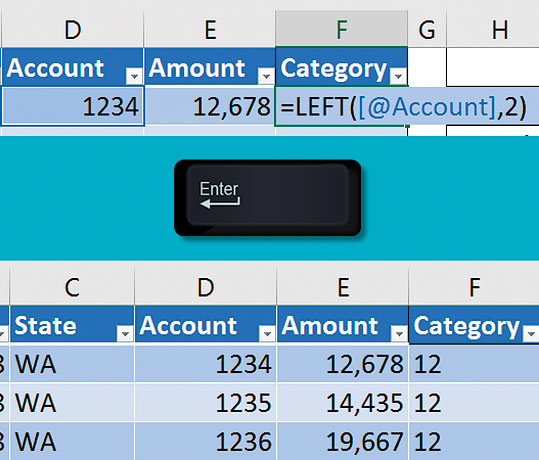
When you create a formula in a column in a formatted table, Excel uses structured references to refer to a cell on the same row. Let’s assume the first two characters in the account number represent a category used for reporting. We can extract the first two characters using the LEFT function.

In Figure 4, I have inserted a new column to the right of the table and entered Category in cell F1. This automatically extends the table to include column F. When creating the formula in cell F2, if you click on a cell in the same row within the table, Excel will insert a structure reference instead of the cell reference as shown in Figure 4. The @ symbol means to extract the value from the same row in a different column, in this case the Account column. The “2” on the end of the formula instructs Excel to extract the first two characters. When you press Enter the formula is copied all the way down the table.    

Range names

Formulas that use structured references quickly expand due to the inclusion of the table and column name. In general, the shorter the formula, the easier it is to understand. 

One way to reduce formula length while keeping the advantages of structured references is to use a range name as an intermediary. Range names can be used to define cells and ranges. They can also be used to refer to structured references.

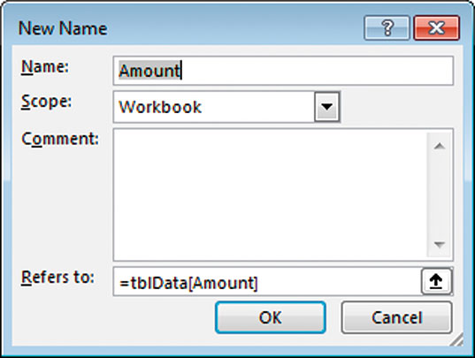
One of the current limitations of structured references is they can’t be used as the source for a Data Validation drop-down list. Range names can also remove that limitation. To create a range name for the Amount column select cell E2 and press Ctrl + Space Bar. This selects all the data rows in the column. Press Ctrl + Alt + F3 to open the New Name dialog. See Figure 5.

The structured reference will appear in the Refers to box at the bottom of the dialog.  Excel will usually insert the column name at the top of the dialog – in this case Amount. If it doesn’t, type Amount as the Name and click OK. We can amend the formula from cell h2 in Figure 3 to =SUM(Amount). Another advantage with using range names is that you can use the fill handle to copy across and the range names won’t change.

Range names can be also used as a source for Data Validation drop-down lists.

Keyboard shortcuts

To apply the default format and create a formatted table press Ctrl + T.

To select just the data in a formatted table press Ctrl + A. To include the heading row, press it again.

To select the current column of data press Ctrl + Space Bar, press again to include the heading. To select the current row, press Shift + Space Bar.

Tab key

The Tab key works slightly differently in a formatted table. Pressing the Tab key usually moves the cell to the right. In a formatted table it will move it to the right until the last column in the table, then it will move down to the cell in the first column on the next row. If you are in the last row and the last column and press the Tab key, a new blank row will be added to the bottom of the formatted table. 

Slicers

Slicers are an easy-to-use graphic filtering interface. They were added in Excel 2010 to filter PivotTables. In Excel 2013 their functionality was extended to filter formatted tables. The Insert Slicer icon can be seen in Figure 1 in the Design ribbon tab.

Resetting a table

Sometimes the functionality of the formatted table can affect other Excel functionality and you may need to remove formatted table features. To do that, right-click the formatted table and choose Table and choose Convert to Range. A dialog will display confirming the change.

Any formulas you had created using structured references will be converted to fixed references. The format remains on the table, but it will no longer update.

The companion video and Excel file will go into more detail to demonstrate these techniques.

Neale Blackwood CPA runs A4 Accounting, providing Excel training, webinars and consulting services to organisations around Australia. Questions can be sent to [email protected]