Excel tips: how to unleash the power of PivotTables

Few people realise that other calculations are built in to PivotTables. People tend to perform many of these calculations outside a PivotTable.

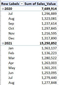
As an example, let’s examine the simple PivotTable in Figure 1.

What if we want to see a running total of sales? This type of calculation is often performed to the right of a PivotTable using Excel formulas.

A running total is built in to PivotTables. Right-click one of the values in the PivotTable and choose Show Values As, then choose Running Total In as per Figure 2. A dialog will open with Date selected. Click OK.

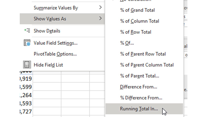
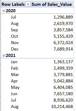
The report changes as per Figure 3. The other reports listed in Figure 2 are worth viewing. Figure 2 shows only a sample of the available reports.

This built-in feature can be impressive. Once people see this report, they often ask if they can also see the monthly value and the running total. They can, but the solution is not intuitive.

The solution is to add the Sales_Value field (column) to the PivotTable again, because you can add a field to the Value section of a PivotTable more than once.

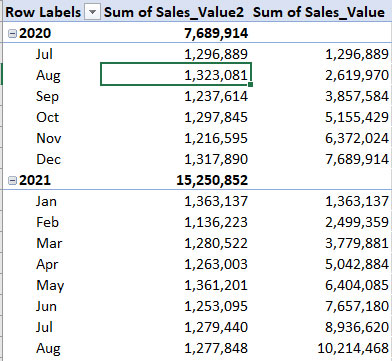
In Figure 4, I’ve added the field again and placed it above the existing field in the PivotTable Field List. This adds the new column to the left of the existing running total column.

You will notice in Figure 3 and Figure 4 that the running total resets each January.

PivotTables are based on calendar years. I have included a technique below to handle financial years using Power Pivot.

While this report is useful, the headings are not. One of the shortcomings of PivotTables is its automated headings. Having “Sum of” and the number added to the headings is not ideal. However, you can edit PivotTable headings.

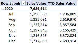
Changing the headings is straightforward. There is only one rule: do not use a name that is also a field (column) name in your data. You can use a space character to change the name. You can add a space character to the end or start of the name. In our case, we can replace

the underscore character with a space to create a more attractive report. See Figure 5.

To create a Running Total for the Australian financial year, we can use Power Pivot and DAX.

Power Pivot with DAX

I covered Power Pivot and DAX in my April 2022 article. That article explains how to enable Power Pivot if you have not already.

Follow these steps to create a YTD running total column for the financial year using DAX.

1. Make sure your data table is in a formatted table. If it is not, press Ctrl + T to convert it to a formatted table.
2. Click inside the table, click the Power Pivot ribbon tab and click the Add to Data Model icon. A new window will open.
3. In that window, click the Design tab, click the Date Table drop-down and click New.
4. This will create a Calendar (Date) table with all the sequential dates to match your data table. In the Date Table drop-down, you can also modify the date range in the future if you need to add more dates.
5. In the Power Pivot window, click the Home tab and select the Diagram View icon at far right.
6. Use the mouse to drag the Date field from the Calendar table to the Date field in the sales data set. This creates a relationship between the Calendar table and your sales data set. Close the Power Pivot window.
7. In the Power Pivot ribbon tab, click the Measures drop-down and choose New.
8. Enter the measure name Total Sales with the following formula
   =SUM(tblSales[Sales_Value])
   At the bottom of the dialog, use the Number format, Whole number with the thousand separator. The name tblSales is the name of my sales data table and Sales_Value is the column name in that table. This measure displays the total sales. Measure names can have spaces in them. Click OK.
9. One advantage of DAX measures is that they can handle different financial years. In the Power Pivot tab, click the Measures drop-down and choose New.
10. Use the name Total Sales YTD with the following formula
    =CALCULATE([Total Sales],DATESYTD('Calendar'[Date],"30/6"))
    This formula takes the Total Sales measure we just created and adjusts it using the DATESYTD function. Using “30/6” on the end specifies the end-of-year date. This measure displays the YTD total sales up to, and including, the month reported. At the bottom of the dialog, use the Number format, whole number with the thousand separator. Click OK.
11. In the Insert ribbon tab, use the PivotTable drop-down to select the Data Model and you can create the PivotTable in Figure 6. This uses the two measures to create a YTD running total based on the financial year. Note: the Date field used in this report is from the Calendar table.

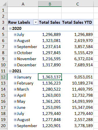
Note: the format we specified for the measures is automatically applied. The headings are more meaningful, no editing required.

Standard PivotTables offer many built-in reports that are hidden in the Show Values As selection. These can save you from having to perform calculations external to the PivotTable.

To handle calculations involving financial years, we can use Power Pivot, the date model, a calendar table and DAX measures.

The companion video and Excel files (Blank and Complete) will go into more detail to demonstrate these techniques.

Neale Blackwood CPA runs A4 Accounting, providing Excel training, webinars and consulting services. Questions can be sent to [email protected]