Excel tips: how to use the Data Model

1 Apr 2022

7 min read time

At a glance

Power Pivot is part of the Excel Data Model. It allows you to report on multiple tables at once and create special calculations called Measures. Measures extend what calculations are possible within Excel’s PivotTable reports, and are written in a language called DAX (Data Analysis Expressions).

The Data Model, Power Pivot and DAX are a huge topic. In this article I will introduce some of the basic features, which are still extremely powerful and flexible. Power Pivot and DAX are also part of Power BI. Anything you learn in Power Pivot can be applied to Power BI.

Loading Power Pivot

To see if you have Power Pivot, click the File tab and then Options (bottom left). Click Addins on the left side. In the Manage: Drop Down (bottom of dialog) select COM Add-ins and click Go. Make sure Microsoft Power Pivot for Excel is ticked and click OK. Power Pivot has its own tab.

Example

We will use four Excel tables, one each for Sales, Dates, Products and Customers. All four tables have been defined as tables using the Format as Table option on the Home ribbon.

Terminology

In Excel tables, we refer to “columns” and “rows”. In databases, these are called “fields” and “records”, respectively.

There are two common table types in the Data Model.

Fact or Data table: This table tends to have the largest number of records, and it may be transaction-based. This table typically has the values you want to report on. In our case, the Sales table is the Fact table.
Dimension or Lookup table: This type of table has fewer records and is related to a specific subject. Each record is dedicated to a single item and has a unique identifier. The Dates, Customers and Products tables are all Dimension tables. There is typically a relationship between each Dimension table and the Fact table. Relationships use unique codes to relate the tables together.

Loading the tables

Click a cell in the Sales table. In the Power Pivot tab, click the Add to Data Model icon. This opens the Power Pivot window. This window can stay open while you continue to work in Excel. If you have two screens, you can have Power Pivot on one screen and Excel on the other. Repeat this step for each of the other three tables.

In the Power Pivot window in the Home tab, click the Diagram View icon (right-hand side of tab). This shows a field (column) listing for each table (see Figure 1).

We need to create a relationship between each Dimension table shown at the top in Figure 1 and the Sales table shown at the bottom. To create a relationship for the Dates table, use the mouse to click, hold and drag the Dates name from the tblDate listing to the Dates name in the tblSale listing. Repeat this step for the Product ID field in tblProduct and the Customer ID field in tblCustomer.

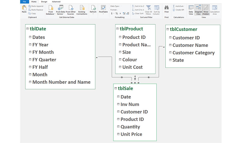
Dimension tables are typically arranged above the Fact tables. Figure 1 shows the view after the relationships are created.

Because we have a Dates table (also known as a Calendar table), we need to define it as a Dates table. This makes many date-based calculations automatic in Power Pivot. In the Diagram View, click the tblDate table, click the Design tab and click the Mark as Date Table icon. Make sure the Dates field is selected and click OK. Now that we have relationships between the tables, we can create a Pivot Table using fields from all the tables.

In the Power Pivot window on the Home ribbon, click the PivotTable icon. Select New Worksheet and click OK. Four tables will be listed in the PivotTable Fields list. Drag the fields as per Figure 2.

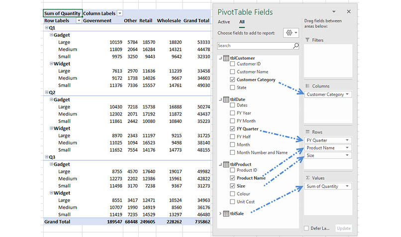
The columns are based on the Customer Category field from the Customer table. The rows are based on fields from the Date and Product tables. The Quantity is a field in the Sales table.

This is a typical report you create when you start using Power Pivot. In a normal PivotTable, you drag fields into the Values section. When using the Data Model, it is best practice to use Measures, not fields, in the Values section.

Measures

A Measure is a named formula that calculates based on its location within the PivotTable. We need to create a Measure for Total Quantity Sold, which adds up the Quantity field in the Sales table.

In Excel, you work with cells and ranges. In DAX, you work with Tables and Table Fields (columns). In the Excel window in the Power Pivot tab, click the Measures drop-down and choose New Measure. Figure 3 shows the entries needed to create a Measure called Total Quantity Sold. When you click OK, the new Measure will appear in the PivotTable. Figure 3 also shows part of the updated report.

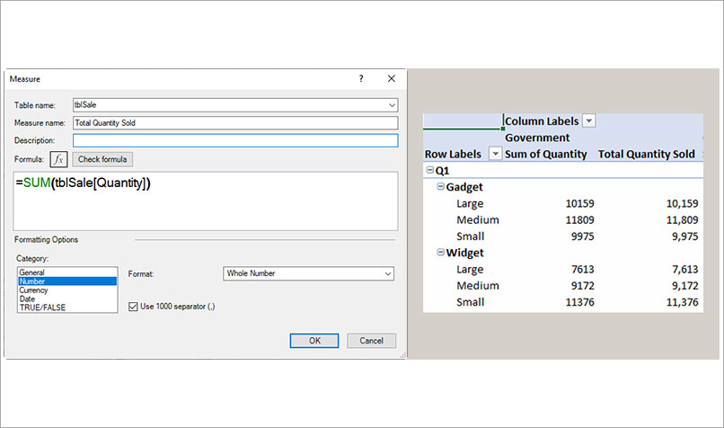
Note that the Measure in the report in Figure 3 is formatted based on the format defined in the Measure dialog. You can click the Check formula button (just above the formula area) to see if you have any errors in the formula. This is more helpful for complex DAX formulas.

We can now remove the Quantity field from the PivotTable. When referring to a table column in a DAX formula, always include the table name. This is best practice for DAX formulas.

SUMX DAX function

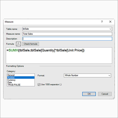
The SUMX function is an iterator function. Iterator functions have the X on the end of an existing function name. This means it can perform calculations based on records (rows) within a table. In our case, we need to work out the total sales for our products. We have the quantity sold in the Sales table and the unit price, but the total sales amount is not included.

The SUMX function can multiply the quantity by the unit price on a row-by-row basis to calculate the total sales value. It then adds up all multiplication results for each row to return a single total value. Use the New Measure option. The settings to use for the Total Sales Measure are shown in Figure 4.

Divide DAX function

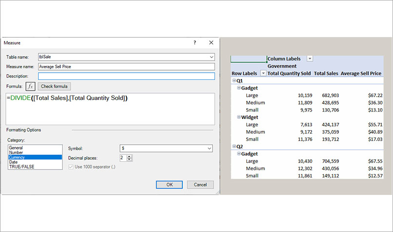
Now that we have a measure for Total Quantity Sold and Total Sales, we can work the average selling price.

DAX has a function dedicated to dividing, and it avoids the divide by zero error. We will use it to calculate the Average Sell Price. Figure 5 shows the settings for the new measure and part of the resulting Pivot Table report. Best practice when referring to measures is to never include the table name. This means that in a DAX formula anything with just brackets around it is a measure. Anything with a table name followed by a name within brackets is a field in a table. This makes editing and understanding DAX formulas much easier.