Loading component...
At a glance
Question
When I link to a cell in a Pivot Table, it inserts the GETPIVOTDATA function. I have tried unsuccessfully to use this function. Am I missing something?
Answer
The GETPIVOTDATA function is very powerful, but has several limitations. As long as you are aware of them, it can provide a way to create flexible reports
Pivot Tables are one of Excel’s most powerful features. Pivot Tables can quickly summarise huge data sets into a table-based report. They can even summarise external databases. If you don’t already use Pivot Tables I highly recommend that you investigate them.
Unfortunately, Pivot Table layouts and formats leave a lot to be desired. In many cases, even though the Pivot Table may contain all the numbers you require, the report itself may not be suitable for presentation. The GETPIVOTDATA function allows you to create a customised report based on the Pivot Table.
Before we look at how to use GETPIVOTDATA, we should first understand its limitations.
- Only values visible in the Pivot Table can be extracted. This means you need to create a Pivot Table that displays all the values you need. You need to ensure that the Pivot Table structure is not modified. Modifying the structure may return an error in existing GETPIVOTDATA functions.
- Pivot Table reports are like web pages, they need to be refreshed to show the latest data. You must ensure the Pivot Table has been refreshed so the GETPIVOTDATA functions return the latest data.
- The first entry in the GETPIVOTDATA function must be text. Unfortunately, Excel won’t accept a reference to a text entry in a cell. I will show you a workaround for this limitation.
With these limitations in mind, you can create a report in the precise layout you require by using the GETPIVOTDATA function.
Syntax
GETPIVOTDATA(Data_Field,Pivot_Table,Field1,Item1,Field2,Item2,…)
Data_Field – the value field you want to extract. Must be a text entry.
Pivot_Table – a cell reference to any cell within the Pivot Table that you want to extract values from.
Field1 – field name that you want to extract from.
Item1 – item name within Field1 that you want to extract.
Fields and Items can be repeated and paired to identify more matches. These define the criteria to report on.
Example
=GETPIVOTDATA("Sum of Sales",Pivot!$A$3,"Region","North","Product","Gadget")
This automatically generated GETPIVOTDATA function will return the sum of the Sales field in the Pivot Table located in the Pivot sheet at cell reference A3, where the Region field contains North and the Product field contains Gadget. Most of the entries are hard-keyed. This formula cannot be copied to other cells to extract other values.
Worked example
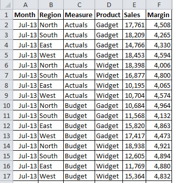
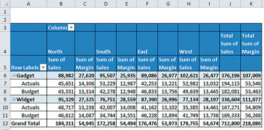
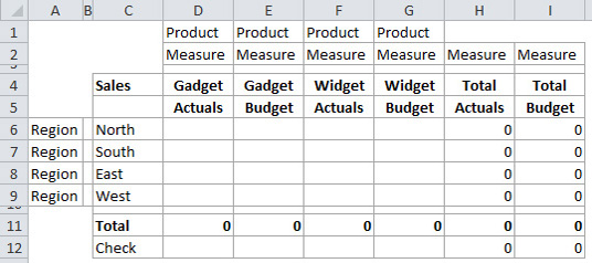
The following example demonstrates the flexibility of the GETPIVOTDATA function. Figure 1 shows an extract of the source data, which contains values for three months. Figure 2 has the Pivot Table and it is in a sheet called Pivot. Figure 3 has the blank report to be populated.
Cell D6 of the report (Figure 3) will contain a formula that can be copied to the other cells in the body of the report. Rows 1 and 2 and column A contain helper cells. Helper cells are not meant to be printed. They simplify creating a flexible formula.
The easiest way to insert a GETPIVOTDATA function is to have Excel create the structure for you. Select cell D6 and press = then navigate to the Pivot sheet and select cell B7 (Figure 2), which has the value that needs to go in D6 of the report. Excel will create the following formula:
=GETPIVOTDATA("Sum of Sales",Pivot!$A$3,"Region","North","Measure","Actuals","Product","Gadget")
We then replace all the text entries in the formula with cell references.
=GETPIVOTDATA(""&$C$4,Pivot!$A$3,$A6,$C6,D$2,D$5,D$1,D$4)
The Data_Field can be either the description as per the Pivot Table, e.g. "Sum of Sales", or the field name in the source data Sales as in this case (column E in Figure 1).
In the formula, the string ""&$C$4 is the workaround mentioned earlier for the text cell limitation. This forces Excel to treat cell C4 as text. The & symbol joins text together.
The $ signs in the formula fix certain rows and columns to allow it to be copied across and down. This formula can be copied to the range D6:G9. Cell D12 in the report (Figure 3) is a check cell. The formula from D6 can be copied to D12 and modified to:
=GETPIVOTDATA(""&$C$4,Pivot!$A$3,D$2,D$5,D$1,D$4)
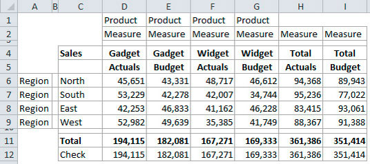
This removes the Region links, $A6 and $C6, and provides the total for Actual Gadget Sales for all regions. This formula can be copied to the cells E12, F12 and G12. The final report is shown in Figure 4.
=GETPIVOTDATA(""&$C$4,Pivot!$A$3,D$2,D$5,D$1,D$4)
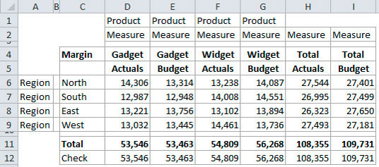
The report’s flexibility is demonstrated when you change cell C4 to Margin. The report updates to display Margin results instead of Sales. See Figure 5.
You may think you could get cell H12 (total actuals for all products) via a GETPIVOTDATA formula such as:
=GETPIVOTDATA(""&$C$4,Pivot!$A$3,H$2,H$5)
The above report could be replicated using the SUMIFS function in Excel 2007 and later and the SUMPRODUCT function in Excel 2003, provided the data is in Excel.
Remember, though, Pivot Tables can summarise external data sources without bringing the data itself into Excel.
Tip
If you need to move a column in between two other columns, you can do it by first selecting the column. Then hold the Shift key down and point the mouse to the right border of the selected column until the arrow cursor shape appears.
Click, hold and drag the column to place it where you wish. Release the mouse, then release the Shift key.

