Loading component...
At a glance
Question
I use the Show Values As option in PivotTables. This converts the report to display percentages of totals.
What I want to do is have both the value and the percentage shown in the PivotTable. Is that possible?
Answer
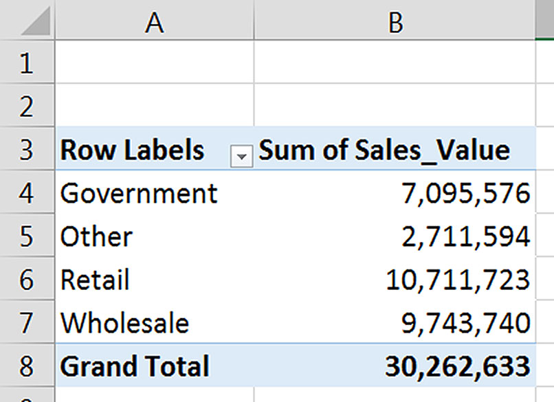
Yes, you can show the values and the percentage on the same report – using the Show Values As option.
Many users are unaware of this useful and underused option. Show Values As is accessed slightly differently in different versions of Excel.
Have a look at the small PivotTable report in Figure 1.
Even though this report is small, the following techniques can be applied to larger PivotTable reports too.
Excel 2013/2016
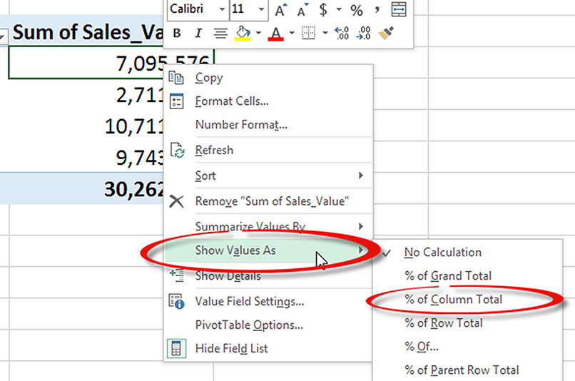
Right click one of the value cells in the PivotTable. One of the options is Show Values As – see Figure 2.
Excel 2007/2010
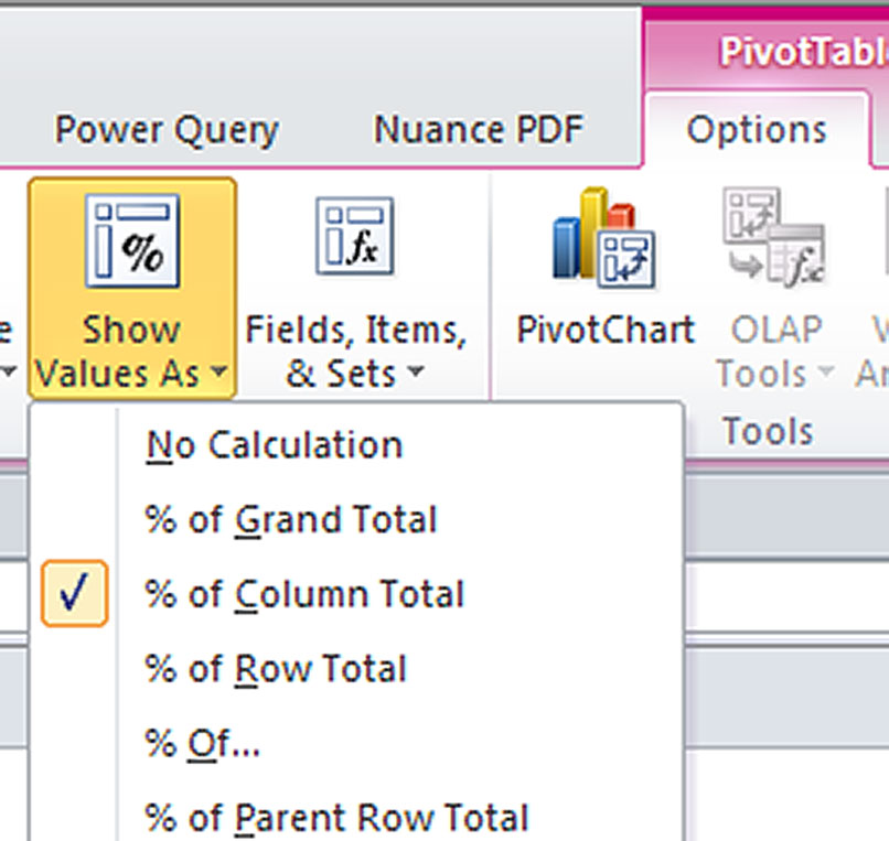
The Show Values As option is in the Options ribbon tab when you select a value cell within a PivotTable – see Figure 3.
Note: There are more options available in both Figures 2 and 3.
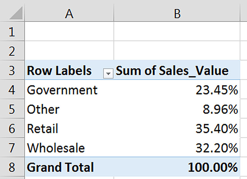
If you select the % of Column Total option, you will amend the report as shown in Figure 4.
The question is, how do you show both the values and the percentages on the one report?
The answer is surprisingly simple, if a little counterintuitive.
You simply drag the values field to the Values area a second time.
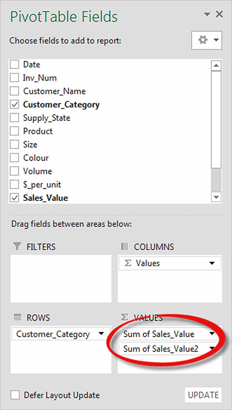
That means the value field is listed twice – see Figure 5.
The first values column of the PivotTable you can leave as values.
You then right click a value in the second value column on the PivotTable and use the Show Values As option to select % of Column Total.
The final step is to change the headings to make them more descriptive.
Unfortunately, the default headings in PivotTables leave a lot to be desired.
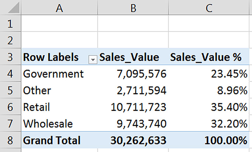
Many users don’t know you can overwrite the heading cells (B3 and C3 in Figure 6).
When changing a heading, you must ensure you do not use an existing field name (column heading) from the source data.
If you do, Excel will stop you and display an error dialog.
If you do want to use a field name, add a space to the end of the name. Excel will accept that.
The amended report with the extra column and updated headings is shown in Figure 6.
You are not limited to adding two value fields.

You can add as many as you need and use the Show Values As options to display different results.
Figure 7 has an example of adding two more columns (Rank and Running Total) to the PivotTable with amended headings.
All these calculations will automatically adjust whenever the PivotTable is refreshed.

The above PivotTables did not have a field in the Columns area of the PivotTable, which helped reduce their size.
Adding fields to the Columns area will increase the complexity of the report, as the new columns will be repeated for each unique entry in the source data field
The Columns area settings are shown with each report – notice the differences.

The sequence of the entries listed in the Columns area adjusts the report layout. Because Size is listed first in Figure 8, the values and percentages are shown under each size.
In Figure 9, the Values item is listed first, so all the sizes are shown under the values and then again under the percentage.
You use the mouse to click, hold and drag the entries to change the sequence within the Columns area.
PivotTable tip
When creating a PivotTable, the values are typically summarised using the SUM calculation. Sometimes a PivotTable will default to the COUNT calculation.
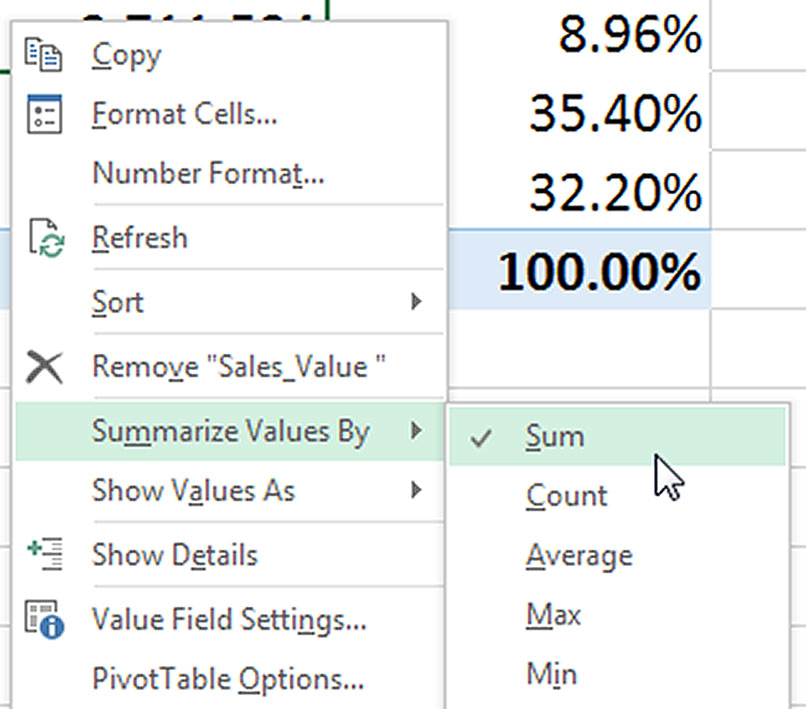
While this is frustrating, it is easy to fix. Right click a value cell within the PivotTable report and choose Summarize Values By and then choose Sum. See Figure 10.
The problem is usually caused by blank cells in the value column of the source data.
A single blank cell in the value column will change the default calculation from SUM to COUNT.
The fix is to populate the blank cells with zeroes. This may sound difficult, but there is an easy way to do this. Follow these steps:
- Select the value range involved.
- Press the F5 function key and then click the Special button.
- Select the Blanks option and click OK.
- Press the zero number key (don’t press Enter).
- Hold the Ctrl key down and then press Enter.
The companion video and an Excel file may assist your understanding.
Neale Blackwood CPA runs A4 Accounting, providing Excel training, webinars and consulting services to organisations around Australia. Questions can be sent to [email protected]

