Loading component...
At a glance
Excel’s IF function allows you to build decision-making into spreadsheets. You can also use IF functions within IF functions, which is called nesting. However, trying to read nested IF functions can be difficult and the logic hard to follow.
To simplify handling multiple conditions, a new function has been added in Excel 2019. It has been available in the subscription version of Office 365 for over a year.
The new function is IFS. Whereas the IF function handles TRUE and FALSE results, the IFS function only handles the TRUE result.
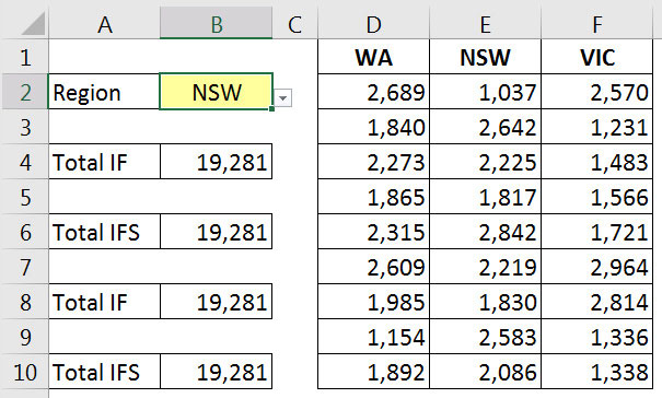
As well as comparing the differences between the two functions, I want to share a little-known technique that can shorten formulas. In Figure 1 there is a drop-down in cell B2 which allows you to select one of the states shown on the right of Figure 1. The drop-down cell determines which column will be summed.
IF syntax
IF (Logical_test, Value_if_TRUE, Value_if_FALSE)
Logical_test is an expression that returns TRUE or FALSE.
Value_if_TRUE can be a value, formula, text or another function.
Value_if_FALSE can be a value, formula, text or another function.
Any text must be enclosed in quotation marks.
Example (not based on Figure 1)
=IF(A1=0,0,B1/A1)This simple example tests cell A1 to see if it equals zero. If it does (its TRUE), then zero is displayed. If it isn’t zero (its FALSE), then B1 is divided by A1. This is a common structure to avoid the divide by zero error.

The formula in cell B4 in Figure 1 has a nested IF function:
=IF(B2=D1,SUM(D2:D10),IF(B2=E1,SUM(E2:E10),
IF(B2=F1,SUM(F2:F10),0)))
The first IF function compares cell B2 against D1. If they are the same, it will perform a SUM calculation on the numbers in column D.
The second IF function is in the Value_if_FALSE section of the first IF function and it compares B2 to the column heading in E1 and performs a SUM if it matches.
The third IF function is in the Value_if_FALSE section of the second IF function and does the final comparison. If it finds a match, it returns the SUM of the value in column F. The zero at the end of the formula is in the Value_if_FALSE section of the third IF function and it is the value displayed if no matches are found. No matches would be found if cell B2 was blank.
It can be difficult to follow formulas when they contain nested IF functions. If there are any more than three or four nested IF functions, it becomes more difficult to understand. That is one of the reasons why IF functions are one of the most common sources of errors in Excel spreadsheets. It is very important to test IF functions for logic errors.
The IFS function
The idea behind the IFS function is to only handle the Value_if_TRUE option and remove the need to nest IF functions.
IFS syntax
IFS(Logical_test_1, Value_if_TRUE_1, Logical_test_2, Value_if_TRUE_2,…)Each Logical_test has its own Value_if_TRUE and you must keep pairing them up in sequence until you cover all the options. See below on how to handle exceptions.
Example (not based on Figure 1)
=IFS(A1=0,0,A1<>0,B1/A1)If A1 does equal zero, zero is displayed. The symbols <> mean “not equal to”, so if A1 is not equal to zero, then B1 is divided by A1. The above formula handles all the possible numbers; i.e. a number is either equal to zero or it isn’t. However, there will be times when you need to handle the “none of the above” situations. We cover that in our Figure 1 example.
The IFS function in cell B6 is:
=IFS(B2=D1,SUM(D2:D10),B2=E1,SUM(E2:E10),B2=F1,
SUM(F2:F10),TRUE,0)
Note there is only one IFS function. The first three Logical_tests have their matching Value_if_TRUE SUM calculations. The TRUE,0 on the end is how you handle exceptions.
If cell B2 was empty, then the first three logical tests would not be triggered and the #N/A error would be displayed. By typing TRUE as the last Logical_test, you handle the “none of the above” situations because you force a TRUE result and can then define the action, a zero, if none of the other logical tests are TRUE.
Little-known technique
Notice how both Figure 1 formulas contain three separate SUM functions. What is not commonly known is that the IF function and the new IFS function can return a range. That means we can move the SUM function to the start of the formula and have the IF or IFS function return a range for the SUM function to calculate. This will shorten the formula.
The rewritten IF formula from cell B4 is in cell B8:
=SUM(IF(B2=D1,D2:D10,IF(B2=E1,E2:E10,IF(B2=F1,F2:F10,0))))
The rewritten IFS formula from cell B6 is in cell B10:
=SUM(IFS(B2=D1,D2:D10,B2=E1,E2:E10,B2=F1,F2:F10,TRUE,0))
Each of the rewritten SUM functions receives a single range or a zero from the IF or the IFS function.
When you use IF or IFS to return a range it must be used within another function that accepts a range, like the SUM function.
The IFS function provides an easier way to create multiple condition formulas by eliminating nesting and hopefully making the formulas easier to read and understand.
Sequence
In both the IF and IFS functions, the sequence that you list the logical tests can be important; both functions are evaluated from left to right. In our example, the sequence wasn’t important as we were looking for exact matches. If you are using “greater than” and “less than” comparisons, make sure you create them in the correct sequence and test the results.
Alternatives
Whether you use a nested IF function or the new IFS function to handle multiple conditions, investigate whether a table structure and a VLOOKUP or an INDEX-MATCH combination might provide a better, more scalable and robust solution.
The companion video and Excel file will go into more detail to demonstrate these techniques.
Neale Blackwood CPA runs A4 Accounting, providing Excel training, webinars and consulting services to organisations around Australia. Questions can be sent to [email protected]

