Excel tips: how to capture logic in a single row

We’ve all seen those formulas that have multiple IF functions nested together. They can make your head spin as you try to follow and understand the logic behind the formula. There is an alternative.

Rather than capturing the logic within each formula, it can be more efficient to capture the logic in a single row or rows, then refer to those rows in your formula. This can simplify the IF function and make it easier to amend the logic in the future. The logic also becomes more transparent to the user.

I’ll use a simple reporting example to show this technique, which can be applied to budgeting, forecasting, or any situation where you need to use the same logic across rows and columns.

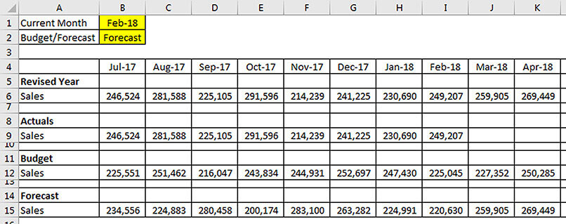
In the example in Figure 1 we have to display the correct Sales figure for each month in row 6. 

The entry in cell B1 determines the current month for actuals. The entry in cell B2 determines the metric to use for future months. Both cells have in-cell dropdowns. 

A typical formula for cell B6 that could be copied across and down would be something like:
=IF(B$4<=$B$1,B9,IF($B$2="Budget",B12,
IF($B$2="Forecast",B15,0)))

The first IF function identifies actuals based on the month in cell B1. The second IF returns the budget figure if Budget is selected in cell B2. The third IF returns the forecast value if Forecast is in cell B2, and it also returns 0 if neither Budget nor Forecast are entered in B2 – that is, cell B2 is blank. 

Centralised logic

By centralising logic you make the logic more transparent and easier to understand, use and change. This involves inserting extra rows that have the results of the logical tests that were shown in the above IF function.

Don’t be afraid to use extra rows in your spreadsheets. If they allow you to simplify formulas, increasing the size of the spreadsheet is worth it. See the Grouping section in this article for a technique to easily hide workings rows.

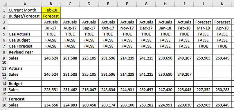
In our example, we need to decide which of the three figures (Actuals, Budget and Forecast) to display in each month. I will insert three rows. These will display whether or not to use each particular figure. Figure 2 has the inserted rows and the formulas in place.

Table 1 shows the formulas in the first column of each of the three new rows.

Cell B5 uses the first logical test from the original IF function to determine if the month is an Actual month.

Cells B6 and B7 use the AND function to review two logical tests. The AND function allows you to review multiple logical tests. The AND function only returns TRUE when all the logical tests return TRUE. If any of the logical tests return FALSE, then the AND function will return FALSE.  

In cell B6 (the Use Budget row), the first logical test makes sure that row 5 has FALSE in it. We only need to use the Budget if the month is not an Actual. The second logical test is the same as the one used in the original IF function to look for Budget in cell B2. Cell B7 is the same as B6, except it is checking for Forecast in cell B2.

The Alternate Formulas in Table 1 take advantage of another logic function called NOT. This simply converts TRUE into FALSE and FALSE into TRUE. Even though it is a simple function, it can be confusing if you are new to logic formulas.

Using descriptive labels makes the logic easier to follow. Using logic like this requires you to get comfortable with displaying TRUE/FALSE in cells. While Yes and No might make more sense, they are not logic keywords.  

The formula that we can now use in cell B9 (cell B6 before the rows were inserted) is much shorter:
=IF(B$5,B12,IF(B$6,B15,IF(B$7,B18,0)))

When you have a logical result in a cell (TRUE/FALSE), you don’t need to test for TRUE, such as, B$5=TRUE, you can just refer to cell B$5. I also added an IF function to cell B3 and copied it across. 
=IF(B5,"Actuals",$B$2)

This makes it obvious what figures are in each column. This row is not used by the other formulas, it is for information only.

When the logic is centralised, you only need to change the logic in one place; you don’t need to find all the formulas that are using the logic. This simplifies maintenance. 

Multiplying by TRUE and FALSE

A little-known technique of logical results is that you can multiply by them. Multiplying by TRUE converts it into 1 and FALSE converts to 0. We can create a shorter formula without an IF function to calculate our sales figure. This technique assumes that the three logical tests are mutually exclusive, which means that only one of them can be TRUE in each column.

The alternative formula for cell B9 is:
=(B$5*B12)+(B$6*B15)+(B$7*B18)

This technique only works for numeric calculations. Since only one of the three cells returns TRUE, only one value will be multiplied by 1 (TRUE); the other two values will return 0 as they are multiplied by 0 (FALSE).

Grouping

You may want to hide these logic rows. The best way to do that is to use Grouping. Select rows 5,6 and 7 and then press Shift + Alt + right arrow. This inserts the Grouping icons on the left, as shown in Figure 3. 

You can click the minus sign to hide the grouped rows and click the plus sign to unhide the rows. Grouping adds visual markers showing that rows are hidden. 

Grouping can also be applied to columns using the same shortcut. 

The companion video and Excel file will go into more detail to demonstrate these techniques.

Neale Blackwood CPA runs A4 Accounting, providing Excel training, webinars and consulting services to organisations around Australia. Questions can be sent to [email protected]