Excel tips: IF function, Group feature and more

1. Is there an easy formula to determine the financial year from a date?

Answer: Assuming the Australian July to June financial year, you can use the following formula to convert the date in cell A1 to the financial year.

=IF(MONTH(A1)<7,YEAR(A1),YEAR(A1)+1)

This is the same formula I shared in August 2005. Notice that the YEAR function is in both the true calculation and the false calculation in the IF function. 

When this occurs, you can usually simplify the IF function as follows.

=IF(MONTH(A1)<7,0,1)+YEAR(A1)

In this case, the IF function is determining the number (0 or 1) to be added to the year of the date in cell A1. As you can see, the second formula is slightly shorter. 

2. I frequently hide and unhide the same set of rows in my sheet, so that the detail does not print on my reports. Is there an easy way to do this?

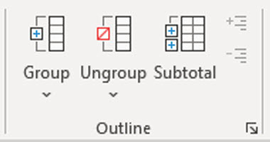
Answer: I always recommend Excel’s Group feature to hide and unhide both rows and columns. The Group icons are on the Data ribbon tab, on the right-hand side – see Figure 1. 

There are also keyboard shortcuts to apply and remove grouping – see Figure 2.

In Figure 3, we want to hide rows 2 to 5 and rows 8 to 11.

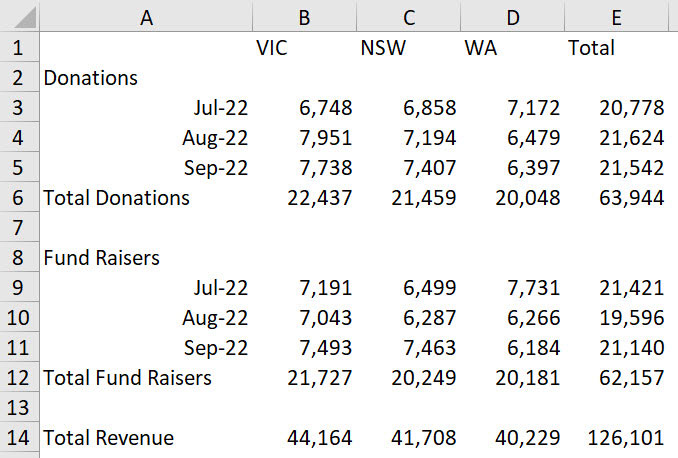
Select rows 2 to 5 and press Shift + Alt + right arrow. Then select rows 8 to 11 and press function key F4. The F4 function key repeats the last action, which in this case can save keystrokes if you need to apply grouping to more rows. 

The amended report is shown in Figure 4.

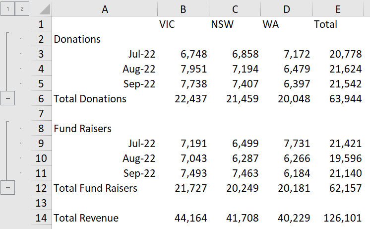
The minus icons on the left of the row numbers allow you to quickly hide the rows. When you hide rows, the icons change to a plus icon. 

Clicking the plus icon unhides the rows. The small 1 (top left corner) hides all the grouped rows. The small 2 shows them all – Figure 5 shows the view when you click the small 1.

Grouping also makes hiding columns easier. Select column B across to column D and press Shift + Alt + right arrow. Figure 6 shows the result.

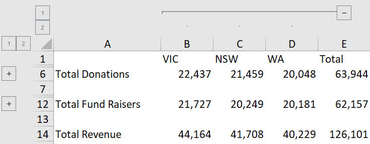
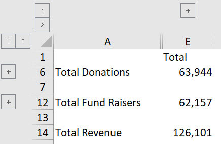
Clicking the small 1 above the column letters results in the report in Figure 7.

Grouping rows and columns is the safest and quickest way to hide rows and columns. The icons are a quick way to hide and unhide rows, plus they provide a visual clue that rows/columns are or could be hidden. 

Removing the grouping removes the icons.

3. Is there an easy way to highlight all the cells that have error messages?

Answer: There are at least two ways to do this. One way is a manual technique, and the other is a conditional formatting technique. I will share another technique that does not involve a format.

Manual technique

The manual technique works once, but it does not update if the formulas change. 

If you are doing a review of an existing file, it might be useful, but if you need this to work as you are developing the file, then have a look at the conditional formatting technique instead.

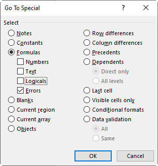
Select the range you want to review. Press the F5 function key. Click the Special button. Figure 8 shows the dialog that opens. Select the Formulas option and untick all the entries underneath except Errors.

Click OK. This selects all the error cells. You can now apply a format and it will be applied to all the error cells. As mentioned, if the errors are corrected the highlighting remains.

Conditional Formatting

This technique is more flexible, and the format updates if the cell’s error is corrected.

Select the range involved. 

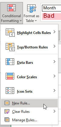
Click the Conditional Formatting icon drop-down in the middle of the Home ribbon and choose New Rule – see Figure 9.

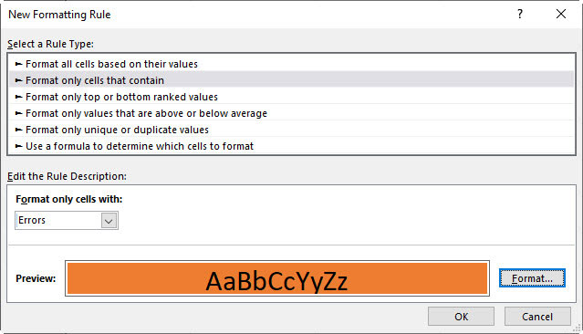
In the dialog that opens, choose the second option from the top “Format only cells that contain” – see Figure 10. 

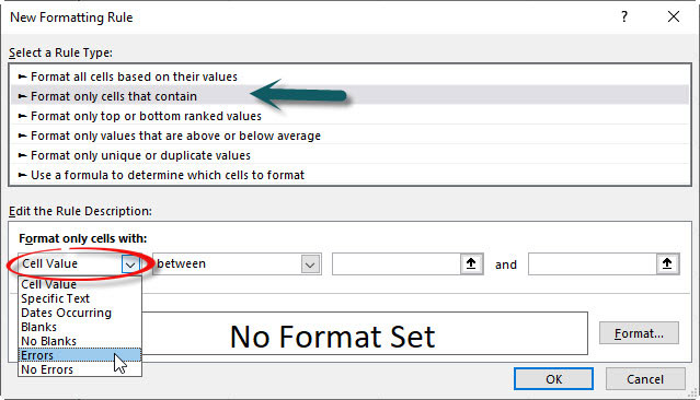
Click the first drop-down and choose Errors. 

Click the Format button, click the Fill tab and choose a colour to fill the error cells (I used orange). Click OK. The completed dialog is shown in Figure 11. Click OK to apply the new rule to the range.

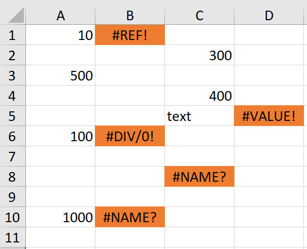
An example of this rule being applied is shown in Figure 12.

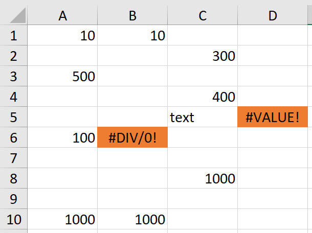
As errors are corrected the highlighting disappears immediately – see Figure 13.

No format technique

As ranges expand, instead of formatting the error cells you could count them instead. If a range has zero error cells, then there is no need to check it.

In the example above, the formula below will count the number of error cells in the range A1:D10.

=SUMPRODUCT(ISERROR(A1:D10)*1)

This formula works in all Excel versions. 

In the latest versions of Excel this formula will also work.

=SUM(ISERROR(A1:D10)*1)

The ISERROR function returns TRUE if an error is encountered. In Excel TRUE = 1 and FALSE = 0. Using *1 on the end within the parentheses converts the TRUE to 1 and sums the number of TRUE (error) entries. 

You may centralise these checks in a validation sheet and have a formula for each sheet in the file.

The companion video and Excel files (Blank and Complete) will go into more detail to demonstrate these techniques.

Neale Blackwood CPA runs A4 Accounting, providing Excel training, webinars and consulting services to organisations around Australia. Questions can be sent to [email protected]