Loading component...
At a glance
Excel has many built-in, automated conditional formats that are great for dashboards and exception reporting. Formulas can also be used to control conditional formats and create formats that work exactly as you require.
Conditional formats are usually based on the value in the cell being formatted, but formulas allow you to format any cell based on the value in any other cell.
When using conditional formatting, it is important to keep in mind that about one in 12 men and one in 100 women have some form of colour blindness. The most common form affects red and green recognition, which makes blue a safer colour to use.
Date example
If we have a list of dates and we need to format the weekend and public holiday dates differently, we can use a formula-based conditional format.
Figure 1 shows the start of a list of dates from the first of the month until the end of the month, as well as a list of public holidays.
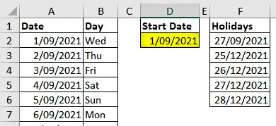
Cell D2 is a data entry cell. Cell A2 has a formula to create the days for the month. The formula has been copied down the column. Column B has a formula that returns the abbreviated day of the week. The companion video to this article goes into more detail about these formulas. It also demonstrates the latest techniques to create sequential dates.
We want to highlight the date and the day in columns A and B when it is a weekend or a public holiday. This technique could also be used to highlight other dates, for example, fortnightly pay dates.
Formula-based conditional formats
This first formula will handle the weekends. Follow these steps to use a formula to create the conditional format.
1. Select the range to work with, in our case A2:B32.
2. Click the Conditional Formatting icon drop-down and choose New Rule.
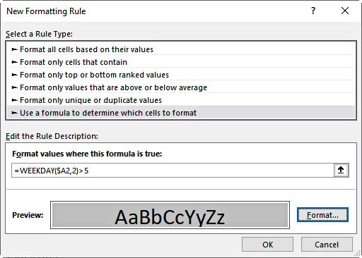
3. Select the last option in the top section, “Use a formula …,” and enter the following formula in the Formula input box:
=WEEKDAY($A2,2)>5
4. The formula you create must return TRUE to apply the format. It acts like the first part of an IF function. This is called a logical test, and it returns TRUE or FALSE.
Click the Format button, click the Fill tab, select one of the grey colours to apply, and click OK.
5. The New Formatting Rule dialog should look like Figure 2. Click OK to apply the format.
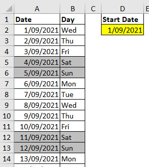
The result is shown in Figure 3.
How does this work?
The WEEKDAY function returns a number (1 to 7) representing the day of the week. Normally you use =WEEKDAY($A2). This returns 1 for Sunday and 7 for Saturday.
When you use =WEEKDAY($A2,2), the “,2” on the end uses a different numbering convention, which is easier to work with. This time, Monday =1 and Sunday =7. This means the formula =WEEKDAY($A2,2)>5 will return TRUE for the weekend days.
The other important part of the formula is the use of the $A2 cell reference. When you create a formula-based conditional format for a range, the reference you use in the formula must relate to the top left cell of the range. Because the formula also handles column B, we fixed the reference to column A using the $ sign. It is common to use trial and error to get the correct formula.
Public holidays
There is no built-in list of public holidays in Excel, so you must create your own. In Figure 1, there are five dates in column F.
Follow these steps to highlight public holidays in blue.
1. Select the range A2:B32.
2. Click the Conditional Formatting icon drop-down and choose New Rule.
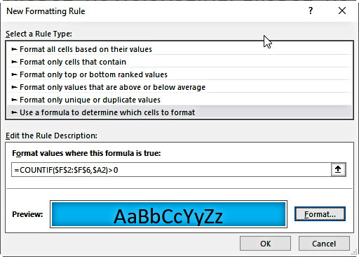
3. Select the last option in the top section, “Use a formula…,” and enter the following formula in the Formula input box:
=COUNTIF($F$2:$F$6,$A2)>0
The COUNTIF function counts the number of times a value appears in a range. If the count is above zero, the value is in the range. COUNTIF uses a fixed range reference, so that the same range is used for the whole conditional format range.
4. Click the Format button, click the Fill tab, select a blue colour to apply and click OK. Figure 4 shows the dialog.
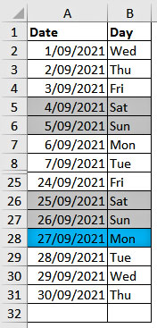
5. Click OK. An abbreviated listing is shown in Figure 5.
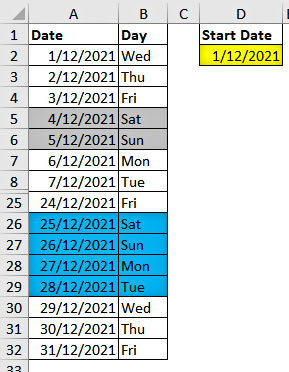
If we change cell D2, we can see the result for December (see Figure 6).
You may want the weekend grey to take precedence over the public holiday blue for 25 and 26 December. You can modify the conditional formats to achieve this.
1. Select the range A2:B32.
2. Click the Conditional Formatting icon drop-down and choose Manage Rules (last option).
3. Click the bottom rule, click the small up arrow on the right of the Duplicate Rule icon and click OK.
Figure 7 shows the amended dialog and the result.

The sequence of the rules is important. The conditions are processed in sequence. If more than one condition applies to a cell, the the first condition listed is applied.
In Figure 7, the grey weekend condition, listed first, overrides the blue public holiday date condition.
There is no practical limit to the number of rules you can apply.
The companion video and Excel files (blank and complete) will go into more detail to demonstrate these techniques.
Neale Blackwood CPA runs A4 Accounting, providing Excel training, webinars and consulting services. Questions can be sent to [email protected]

