Excel Tips: Automated row hiding in Excel reports

2 Sep 2024

5 min read time

At a glance

There is often a need to hide zero and blank rows in Excel reports. This process can be automated by combining a formatted table, formulas, a slicer, and a text box.

To demonstrate the technique, I will use a report from a previous article – see Figure 1.

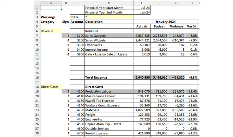
The blank rows (12 to 15) in the report allow you to add new account numbers. These blank rows should be hidden for the purposes of displaying or printing the final report.

Note row 27. In this row, account number 4600 Outside Services has no actuals or budget values. Ideally, this row should also be hidden.

To enable this technique insert five columns on the left of the report – see Figure 5.

In Figure 2, four columns (A to D) have been defined as a formatted table. This enables the use of a slicer to filter the table and the report.

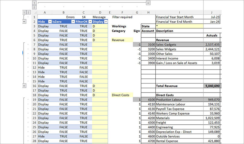
Column E is blank and separates the formatted table from the report.

The Display column (column D) allows you to control the rows that must be displayed. The yellow input range gives you the option to enter a D to ensure certain report rows are always displayed.

The IsZero column (column B) determines if the report row has blanks and/or zeros. The formula in cell B3 is:

=COUNTIF(J3:Z3,0)=COUNTA(J3:Z3)

This formula returns TRUE if the report range (columns J to Z) only contain blank or zero cells.

The COUNTIF function counts how many zeros are in the range. Note a blank cell returns zero. The COUNTA functions returns how many entries are in the same range. If the two functions return the same value, it means all the report entries are blank or zero and the row needs to be hidden.

Column A determines whether to display or hide the row. The formula in cell A3 is:

=IF(AND([@IsZero],[@Display]=""),"Hide","Display")

The square brackets are called structured references. They reference a specific column within the formatted table. The @ symbol means refer to the same row in the other column.

The AND function returns TRUE if TRUE is in IsZero column (column B) and if the Display column (column D) is empty. If column D has an entry or column B has FALSE, then the AND function will return FALSE.

If the AND function returns TRUE then the word “Hide” is returned, otherwise the word “Display” is returned.

Slicer

Slicers are graphic objects that simplify filtering a formatted table or a PivotTable report.

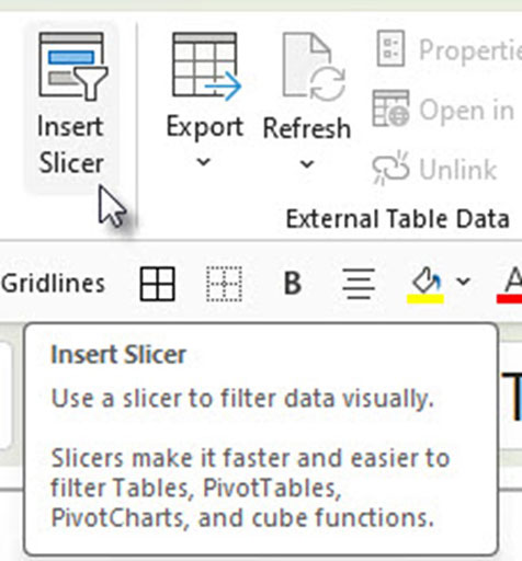
To add a slicer to a formatted table, select a cell within the table and click the Table Design tab. Click the Insert Slicer icon – see Figure 3.

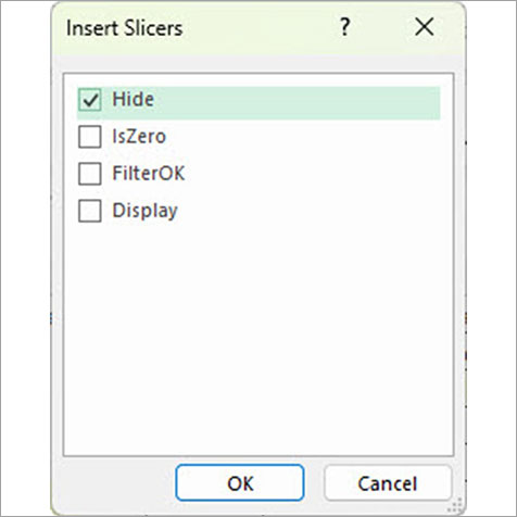
In the dialog that opens, tick the Hide column and click OK – see Figure 4.

Slicers usually list items vertically. To better fit the report layout, the slicer needs to list them horizontally.

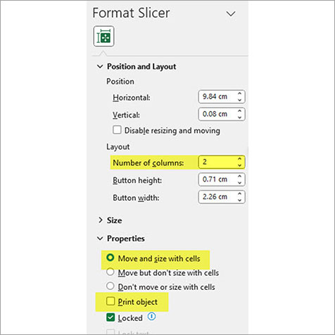
To change the setting, right-click the slicer and choose Size and Properties (see Figure 5). In the Task Pane on the right of screen open the Position and Layout section. In the Layout section enter 2 in the Number of columns box.

In the Properties section, select the Move and size with cells option and untick the Print object option. These settings move the slicer if the columns on the left are hidden and stop the slicer from printing.

Resize the slicer to fit across the top of the report as shown in Figure 6.

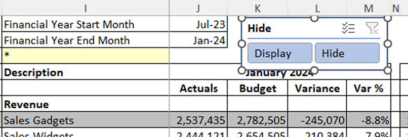
Two further changes are needed to make the slicer easier to use.

The first is the multi-select setting. This is the three-ticks icon on top right of the slicer. Click that icon to activate the multi-select option.

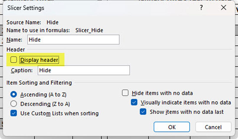
The other setting removes the slicer heading. Right-click the slicer and choose Slicer Settings. Untick the Display header option and click OK – see Figure 7.

The final slicer is shown in Figure 8.

Clicking the Hide button on the slicer hides the blank and zero rows in the report – see Figure 9.

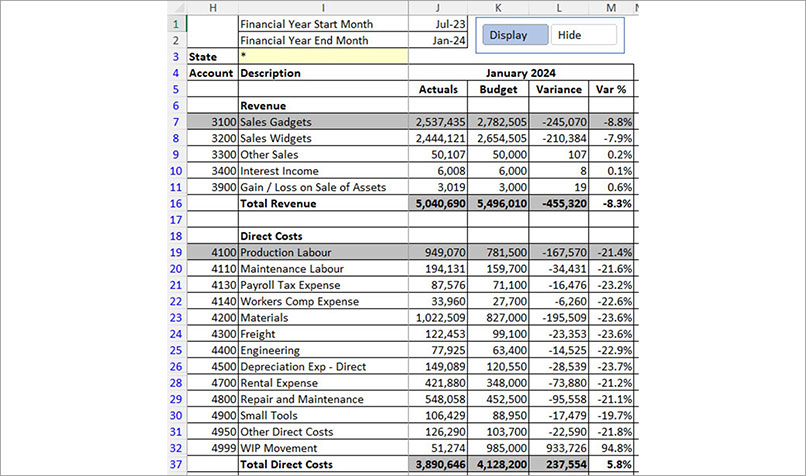
Note: blue rows numbers mean a filter is in place. Row 27 has been hidden.

How to identify filter errors

Unfortunately, filters don't automatically update when values change. This potentially means a row that should be visible is hidden.

As an example, account number 4600 on row 27 has zero values and is hidden. If the data is amended to include a value for 4600 the filter won’t update, and the row remains hidden. The Hide button on the slicer must be clicked twice to re-apply the filter.

The SUBTOTAL function can perform calculations on visible cells.

In the FilterOK column (column C) the formula in cell C3 is:

=SUBTOTAL(3,[@Hide])=IF([@Hide]="Display",1,0)

The SUBTOTAL function returns 1 if the row is visible and 0 if the row is hidden. The IF function checks if that result is correct.

This formula returns TRUE if Display is in column A and the row is visible. It also returns TRUE if column A displays Hide and the row is hidden.

The formula returns FALSE if Display is in column A and the row is hidden or if column A has Hide and the row is displayed.

The formula to check all the entries in the FilterOK column in cell C1 is:

=COUNTIF(tblDisplay[FilterOK],FALSE)

This is another example of a structured reference. The table name tblDisplay is followed by square brackets around the column name. The table name is required when referring to a table column outside the formatted table.

This formula counts the number of times FALSE appears in the FilterOK column. If it is zero, then all the rows are displayed correctly. FALSE in column C means the filter to that row needs to be re-applied.

The formula in cell F1 displays a message for the user:

=IF(C1=0,"OK","Filter required")

A text box on the report has been linked to cell F1 – see Figure 10.