Excel tips: how to use dynamic arrays' new functions

Dynamic arrays are a new feature in Excel 365 (subscription version). At present, the feature is only available to those who have the monthly update channel. These features will be made available to other Excel 365 users in July 2020. Older Excel versions will not receive this functionality.

Unique function

This function extracts unique entries from a list. It works on single or multiple column ranges. It also handles two versions of UNIQUE. The default version removes duplicates.

It can also list entries that only appear once.

Syntax

Note: when reading Excel’s formula syntax, any arguments within square brackets are optional. When omitted, their default value is used. UNIQUE(array,[by_col],[exactly_once])

array – the range to extract UNIQUE entries from. This is typically a vertical list, but it can also be a horizontal range. If it is horizontal, you need to enter 1 or TRUE in the by col argument that follows.

by col – optional – enter 1 or TRUE to specify a horizontal range to extract from. If omitted, the default is FALSE, which specifies a vertical range.

exactly once – optional – enter 1 or TRUE for the function to return only entries that occur once in the array. If omitted, the default is FALSE, which instructs UNIQUE to remove duplicate entries.

In most cases, the two optional arguments would not be used. Most lists that you will extract from are vertical. In most instances, you would need to remove duplicates, rather than show the entries that appear only once.

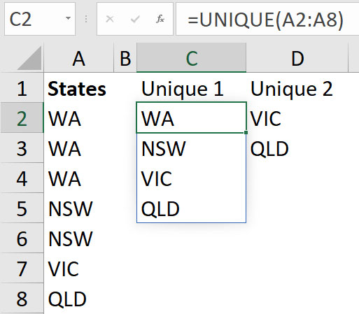
Figure 01 shows the two variations of UNIQUE. As explained in the previous article, these new functions automatically spill into other cells. Formulas are entered in the top left cell of the range. 

Cell C2 has the default treatment and removes duplicates. The formula spills down the range.

Cell D2 uses 1 for the exactly once argument. Its formula is

=UNIQUE(A2:A8,,1)

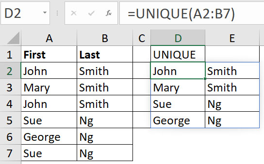
Figure 02 illustrates how multiple columns are treated.

There are two duplicated names in the list; they have been ignored for the UNIQUE list. Note: the function spilled across two columns because the range selected had two columns. The formula was entered in cell D2.

Filter function

You can now filter dynamically via a function. This opens up many possibilities for adding interaction to reports and dashboards.

Syntax

FILTER(array,include,[if-empty])

array – the range to filter.

include – the condition/criteria to use to determine which rows to display.

if-empty – optional – what to display if the FILTER condition returns no rows. A text string is typically enclosed in quotation marks. If you need to display separate text messages across columns, you need to use array syntax. If you wanted to display None in column 1, Nil in the column 2 and 0 in column 3, you would use {“None”,”Nil”,0}.

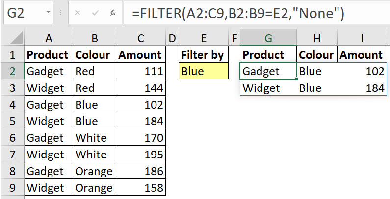
Figure 03 shows an example of the FILTER function in action in cell G2.

The entry in the include (second) argument is worth examining.

B2:B9=E2

This type of logical test was not possible in most formulas before dynamic arrays were introduced. This structure returns eight separate TRUE/FALSE results, one for each cell in the range B2:B9. If the result is TRUE, the row is displayed. Note: logical tests are not case-sensitive.

To see how this works, select just the argument in the Formula Bar and press the F9 function key. Figure 04 shows the results. Press Esc afterwards, or the captured results remain.

The two blue entries in cells B4 and B5 are in the third and fourth cells within the range. They both display TRUE; all others display FALSE.

If no rows match the condition, the word None appears in cell G2.

Multiple filter conditions

The include (second) argument can handle multiple conditions. You need to use parentheses and the * or + signs to create the condition. When you create a condition or criterion, you need to use a logical test to return TRUE or FALSE. When using multiple conditions, there are two types of comparisons.

AND comparison

If you have two conditions and you want to display the row if both conditions are met, then you are using an AND comparison. The structure to use for this type of comparison is shown in Figure 05.

The formula in cell H2 is displaying the row if the colour is Red and the value is above 140. You need to enclose the logical tests within parentheses (brackets) and separate them with the * (the multiplication symbol). In Excel, TRUE = 1 and FALSE = 0. When you multiply the results together, if either of the logical tests is FALSE (0), then that will return zero or FALSE. Both logical tests must return TRUE (1) so that 1 times 1 equals 1, which is the same as TRUE.

OR comparison

If you have two conditions and you want to display the row if either condition is met, then you are using the OR comparison. The structure to use for this type of comparison is shown in Figure 06.

The formula in cell G2 displays the row if the colour of the row is either Red or White. By using the plus symbol between the parentheses, you add the results of each logical test. Since both conditions relate to colour, the highest value you can achieve is 1 per row because a colour can’t be both Red and White. Hence these conditions are mutually exclusive. If both logical tests are FALSE, then the result is zero and treated as FALSE, and the row won’t display.

OR comparison across columns

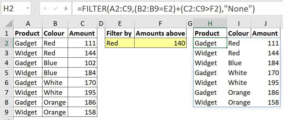
Let’s return to the AND example and convert it into an OR comparison. We now want to display the row if the colour is Red or the amount is above 140. Figure 07 shows the result. As we can see, the only row that isn’t displayed is row 4, because it doesn’t meet either criterion.

The multiple criteria result for row 3 is worth noting. It returns 2 since the row is both Red and the amount is above 140. The 2 result is treated as TRUE and the row is displayed. Excel treats any positive number as TRUE, and zero is always treated as FALSE.

Being able to dynamically return a filtered list or table using formulas offers many options for adding user interaction to reports and charts. Note: Office 365 has been recently renamed as Microsoft 365.

The companion video and Excel files (blank and complete) will go into more detail to demonstrate these techniques.

Neale Blackwood CPA runs A4 Accounting, providing Excel training, webinars and consulting services to organisations around Australia. Questions can be sent to [email protected]