Excel tips: how to capture errors using a centralised validation sheet

Spreadsheets are prone to errors, and part of the creation process is building in validations to capture errors. Some errors are identified and fixed in the development process. Others are part of the normal operation of the file and need the user to identify and fix them, for example, adding new account numbers or departments.

I recommend including validations close to the figures being validated, but as spreadsheet files typically have many tabs, checking all the validations may be time-consuming. You also need to ensure all validations are reviewed. If there are validation errors, you need to know what they are, where they are, and how much they are. 

To solve these issues, I recommend including a centralised validation sheet. This sheet has direct links to all the validation cells and lets you check all the validations in one place.

Validation techniques

Differences

Some validations can be as simple as deducting one number from another. If the numbers are validated as correct, the resulting difference should be zero. The problem with this method is that it can be difficult to scan large ranges to ensure all cells are zero.

Conditional format 

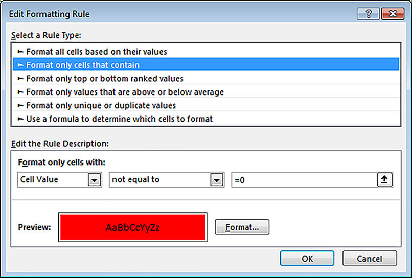
To make it easier to identify non-zero cells, you can use a simple conditional format as shown in Figure 1. Select the range involved, then click the Conditional Formatting icon on the Home ribbon and click New Rule. This rule highlights all non-zero cells in red.

Warning: A cell displaying zero may be highlighted if it contains a small fraction and the format doesn’t show it.

Logical tests for validations

An alternative or a companion to the difference calculation is a logical test. A logical test is usually the first argument in an IF function but it can be used in a cell by itself. It is a formula that returns TRUE or FALSE. A simple logical test is:

=A1=B1
This formula will return TRUE if A1 and B1 are the same and FALSE if they are different.

When I use logical tests in my validations, I set up the formulas so that TRUE is valid and FALSE is invalid. Logical tests can simplify handling large numbers of validations.

Rounding

Most validations can be related to zero: you deduct one figure from another and the difference should be zero. However, many files use some sort of rounding. When validating rounded numbers the tolerance is usually 1. Typically you have to check if the difference is between -1 and 1. You can use the ABS function and the IF function to simplify this check.

ABS function

The ABS function is a mathematical function that, in practice, converts negatives into positives and leaves positives unchanged. Instead of testing if a difference is between -1 and 1, you can test for less than or equal to 1. The formula below returns TRUE if the values in A1 and B1 are within 1 of each other, and FALSE if not:

=ABS(A1-B1)<=1

IF function

If you prefer to display text instead of  TRUE/FALSE you can use an IF function as shown below:

=IF(ABS(A1-B1)<=1,"OK",”Error”)

Another alternative is to show the difference instead of the word:

=IF(ABS(A1-B1)<=1,"OK",A1-B1)
In this case, OK is displayed when the values in A1 and B1 are within 1 of each other. If the difference is greater than 1, then the difference is displayed.

If you have already identified differences in your model, you could add another row with logical tests and link those to your centralised validation sheet. Using TRUE/FALSE has advantages when creating an overall validation formula.

Overall validation

When you have used TRUE/FALSE results for your validations, it is a simple process to create an overall validation formula to examine all the validations. An overall validation can be linked to all the major sheets in the file, so you can immediately see when an error occurs. 

Assuming you have a centralised validation sheet, with TRUE/FALSE validations in the range B2:Z100, The following formulas can be useful.

=COUNTIF(B2:Z100,FALSE)
This counts how many validation errors there are.

=COUNTIF(B2:Z100,FALSE)=0
This will display TRUE if there are no errors and FALSE if there are any errors.

=IF(COUNTIF(B2:Z100,FALSE)=0,"OK","Error")
This will display the word Error if there are any errors and OK if not.

How to solve rounding problems

I am not aware of a one-size-fits-all rounding solution for Excel. There are two common issues:

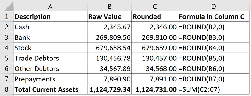
• the sum of the rounded detail values doesn’t match the rounded total, see Figure 2 (above)
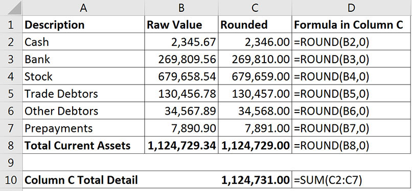
• the total figure of the rounded values is not the sum of the rounded values, see Figure 3

The following technique, which uses a balancing item, ensures the total is rounded correctly and the rounded detail values add up to the rounded total. Note, however, that this solution may not be suitable to use in all situations.

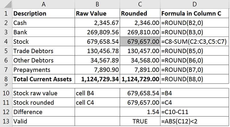
This technique, shown in Figure 4, requires you to identify a detail value that will be used as a balancing item. Typically, you use the largest value in the range. This value is used to make sure the rounded detail equals the rounded total.

This balancing item contains a formula that deducts all the other rounded detail values from the rounded total (cell C4 in Figure 4).

You need to validate the balancing item rather than the total. The balancing item must be within the accepted rounding tolerance. I have used a rounding tolerance of 2 (cell C13), because all the detail values in the range were rounded up.

Rounding tolerance

The typical rounding tolerance is 1 unit, but there are times when most numbers in a range will be rounded up or most rounded down, as in Figure 4. This can cause a difference of more than 1. It can be useful to have a central input cell for the rounding tolerance value. It is usually set to 1, but if you have the occasional differences of 2, you can change the tolerance cell to 2 and all the validations should become valid.

All the validation formulas need to compare differences to this central tolerance cell value, rather than a hard-keyed 1. I typically use a range name for the tolerance value, as this makes it easier to use in formulas. 

Tips for a centralised validation sheet

Quick linking
When compiling a centralised validation sheet, you can save time by using the following technique. Once you have created a range of validations in a sheet, select the range and copy it, then go to the central validation sheet and select a blank cell. Press in sequence Alt H V N. This is a shortcut for Paste Link, which is in the Paste Special dialog. Paste Link creates links to all the individual cells in the copied range. You can then add a descriptive label for the new range of validations. Repeat this for all the validations in the file.

Navigation shortcut
Once you have centralised links to the individual sheet validations, you can use two shortcuts to navigate quickly between sheets. In the centralised validation sheet, select a linked cell and press Ctrl + [ to take you to the validation cell. To return to the central validation sheet, press in sequence the F5 function key, then Enter.

The companion video and Excel files (File 1 and File 2) will go into more detail to demonstrate these techniques.

Neale Blackwood CPA runs A4 Accounting, providing Excel training, webinars and consulting services to organisations around Australia. Questions can be sent to [email protected]