Excel tips: how to deal with dynamic arrays

My first Excel article was published in May 2002, and it covered Control key shortcuts. Eighteen years later, and May 2020 marks my 200th Excel article, which covers a new feature that will revolutionise how Excel is used. This is the first of three articles on this new feature called dynamic arrays.

Versions

Office 365 is Microsoft’s subscription version of its flagship Office suite of products. Currently, this subscription version is being updated with new features that won’t appear in the current full version of Office 2019 (DVD version). These new features will be included in the next full version, estimated to be Office 2022.

The full versions receive updates, but they are bug or security fixes, not new features. In this way Microsoft hopes people will move to the subscription version to get the new features sooner.

My subscription version is on the monthly update cycle, and in January this year I received the update that included dynamic arrays. Those whose subscription updates six-monthly should receive the update in July 2020.

You may have heard of, or even used, array formulas. These advanced formulas allow you to create complex condition-based calculations. With the release of dynamic arrays, array formulas are redundant. If you have used arrays in the past, you will be well- positioned to make the most of dynamic arrays. Dynamic arrays make array functionality easy to access for all users.

Changes to formulas

Microsoft has changed Excel’s calculation engine to incorporate dynamic arrays. It has added a new symbol and more error messages to handle the new features. When explaining and demonstrating these new features, I will use the following terms:

new (with dynamic arrays)
old (before dynamic arrays)

To explain and demonstrate this new feature, we will use a simple but powerful example. Some of the magic of these new features is only apparent when watching the companion video. “Automagically” could soon become a word; many of these features seem like magic. As the renowned science fiction writer Arthur C. Clarke said: “Any sufficiently advanced technology is indistinguishable from magic.”

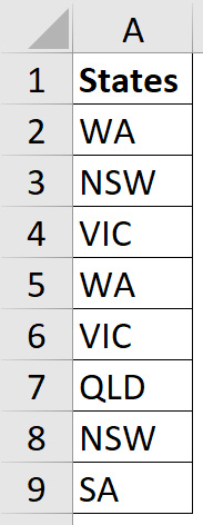
In Figure 01, we have a simple list of duplicated states.

It is common to want to extract the unique entries from a list of duplicated entries. In the past, this required macros, advanced filters or pivot tables. There is now a function that does it automatically.

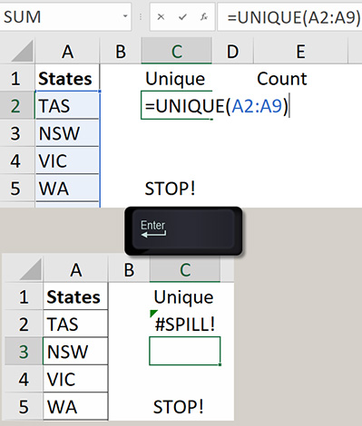
In Figure 02, we can see a new function in action. 
In cell C2 I typed:
=UNIQUE(A2:A9)

When I pressed Enter, the rest of the range was automatically populated with the unique state entries from the range A2:A9. They appear in the same sequence as they occur in the list.

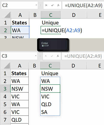
Three things to note in Figure 02:

1. The light blue line around the range C2:C6.
2. The bottom image of Figure 02 has the active cell as C3 – note the font colour in the Formula Bar at the bottom compared to the top. The bottom formula seems faded – it’s light grey.
3. No $ signs used.

Spilling the bean counters

The blue outline is called the Spill range. This is a totally new concept in Excel. A Spill range will expand or contract based on the formula in the top left cell of the range. Spill ranges can also go across rows and columns (two-dimensional).

There is a single formula in the Spill range. It is in the top left cell of the range. If you click another cell within the Spill range and then click the Formula Bar (or press F2), it will be blank. The Formula Bar shows the formula as light grey when the cell is selected, as per the bottom image of Figure 02.

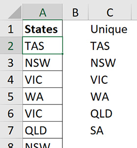
If I change cell A2 to TAS, the UNIQUE function will automatically update. See Figure 03.

Adding an entry below the list in cell A10 won’t update the UNIQUE result as the range is set in the formula to A2:A9. It would automatically update if you had referred to a column range within a formatted table. Formatted tables automatically expand to include extra rows.

Lack of $ signs

Since the formula is only in the top left cell of the range, no $ signs are required to fix the range reference.

Referring to a spill range

You can refer to the Spill range using a new formula symbol. Let’s say we want to count how many unique states there are. The COUNTA function counts all entries. In cell E2, I have entered the following formula using the new # symbol:

=COUNTA(C2#)

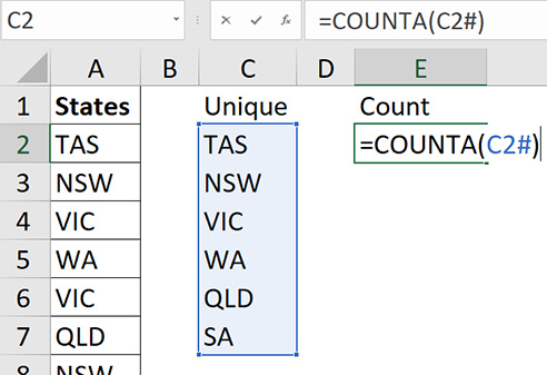
This function references the top left cell of the Spill range, followed by the # symbol. The # symbol instructs Excel to refer to the Spill range that starts in cell C2, as you can see in Figure 04. This range will automatically expand or contract depending on the formula in cell C2.

Spilling issues

When I entered the original formula, there was nothing under my formula in cell C2. If there was an entry that would be overwritten by the Spill range, then a new error appears in the cell when I press Enter: the #SPILL! error. See Figure 05.

As soon as you delete the entry in cell C5, the Spill range will automatically populate.

Existing functions can now perform magic

There are six new functions that work with dynamic arrays. We will look at the other five, plus revisit UNIQUE in the coming articles. Dynamic arrays also impact how existing functions work.

Let’s say we want to count how many characters are in the range A2:A9. Normally, this would involve entering another column with a LEN function in each cell next to column A. The LEN function counts the length of a text string. We would then use a SUM function to add up all the LEN function cells. 

With dynamic arrays, we can use a single formula to find the total number of characters in the range.

In Figure 06 I have entered the following formula in cell G2: =SUM(LEN(A2:A9))

With dynamic arrays, when a function refers to a range it is as if the function is performing its calculation on each separate cell within the range. This is how array formulas worked in the old versions.

In this case, each cell in the range A2:A9 has its LEN result calculated. The SUM function then adds up all the LEN results to arrive at a total number of characters in the range.

Compatibility issue

If you enter the formula from G2 in the old Excel, the result would be 3. 

When you refer to a range within a function that normally accepts a cell, Excel will refer to the corresponding row (or column) from the range referred to.

In the case in Figure 06, cell G2 would refer to cell A2 – hence it would return 3 for TAS. If you refer to a range that doesn’t have a corresponding row number, the #VALUE! error is returned.

You can still access the old-style referencing.

@ symbol

The @ symbol is used to force Excel to use the old-style referencing used before dynamic arrays. The @ symbol is also currently used in formatted tables references. It means to refer to the corresponding row within the table.

When you eventually upgrade to the new Excel, you may find the @ symbol inserted in your formulas to represent the old-style referencing.

The companion video and Excel file will go into more detail to demonstrate these techniques.

Neale Blackwood CPA runs A4 Accounting, providing Excel training, webinars and consulting services to organisations around Australia. Questions can be sent to [email protected]