Excel tips: How to do dynamic arrays (subscription version)

Dynamic arrays were introduced to Excel in 2020, and offer a new way to perform calculations. I covered them in three consecutive articles in 2020.

One problem they had when first implemented was an inability to easily SUM individual columns or rows within the dynamic array. This has been solved by a recent update in the subscription version of Excel.

This solution requires the subscription version, which has the new LAMBDA function. LAMBDA was explained in my June 2020 article.

Worked example

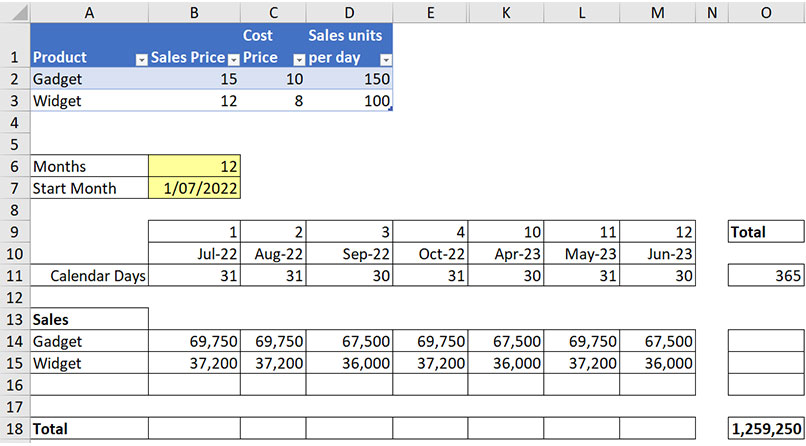
Let’s look at a simple budget example. Figure 1 shows the input table at the top of the sheet, with a simple sales budget created underneath it. The table is named tblSales.

I have hidden the middle months (Nov-22 to Mar-23) so the image displays better on the page.

Dynamic arrays allow you to use a single formula to populate a range. That range may be vertical, horizontal or two-dimensional. The formulas used in Figure 1 have examples of all three types of ranges.

Table 1 shows six dynamic array formulas and their descriptions. They are explained in more detail below.

The SEQUENCE function used in cell B9 generates the numbers 1 to 12. It also controls how many other columns are populated by subsequent formulas. The SEQUENCE function “spills” to the right to populate all 12 numbers.

The term “spill” is related to dynamic arrays, which can spill to the right, down or in both directions. A single formula populates a range. In a spill range, the formula is only in the to, left cell of the range.

Changing cell B6 to 10 would stop the SEQUENCE function in cell K9. The other monthly formulas would also stop at column K. Columns L and M would be blank.

The EDATE function increments a date by a number of months. The first argument is the start date. The second argument is the number of months to add.

In cell B10, we use the start date from cell B7 and add the month numbers from cell B9 and deduct 1. This ensures we start with July 2022. The reference B9# refers to the spill range.

You add the # (hash) symbol to the end of the cell reference in the top, left of the spill range. This forces the formula in cell B10 to spill across to the right to match the entries in row 9 and create the other month headings.

The DAY function in cell B11 returns the day number from a date.

The EOMONTH function returns the last calendar day of the month selected.

This function combination returns the number of calendar days in the month.

The +0 in the formula in cell B11 fixes a date bug that is currently in dynamic arrays. Sometimes a date generated by a dynamic array is not recognised as a date. It is converted into a date by performing a basic calculation, like adding zero to it.  Referring to B10# is all that should be required, but that returns an error. Using B10#+0 fixes the error.

Using zero on the end of EOMONTH means add zero months to the start date supplied by B10.

The formula in cell A14 is called a structured reference. Structured references refer to formatted tables. In this case, it refers to the product column in the table at the top of the sheet. The two product names are returned from the table. The formula spills down as far as required to display all the products.

The SUM in cell O11 adds up the calendar days based on the spill range starting in B11.

The SUM in cell O18 adds up all the allocates sales based on the spill range starting in B14.

There is a single formula in cell B14, which allocates the budget sales between products and across the months. It spills down and across. The formula is

=tblSales[Sales Price]*tblSales[Sales units per day]*B11#

There are two structured references, one to extract the Sales Price from the table and one for the Sales units per day. These two references cause the formula to spill down to match the number of data rows in the table.

The two table references are multiplied together and multiplied by the number of days from cell B11. By using the reference B11# we force the formula to also spill across to the right. This creates a two-dimensional range from a single formula.

Summing problem

We need to add up the columns and rows of the sales allocation range B14:M14. This ability has been lacking in dynamic arrays up until the recent update. There was a complex solution, but it was not easy to explain or understand.

You would think that we could use the following formula in cell B18 to sum July’s sales and spill across for the other months.

=SUM(B17#)

Unfortunately, this doesn’t work. It sums up the whole two-dimensional range rather than just  column B in the range. It also doesn’t spill across. This formula is used in cell O18 to add up the whole sales allocation range.

A solution has been provided by the new function BYCOL, which allows you to access each column within a two-dimensional range. BYCOL requires the use of the LAMBDA function as the second argument to perform a calculation.

The formula for cell B18 that spills across and sums all the columns is

=BYCOL(B14#,LAMBDA(x,SUM(x)))

BYCOL extracts each column from a range and transfers it to the x variable in the LAMBDA function. The SUM function within the LAMBDA function uses that x range and adds up the column. Because B14# is used, the formula spills across to match each column of the spill range. Each column is summed separately.

There is a new BYROW function as well. It also requires LAMBDA as its second argument. The total formula for cell O14 is

=BYROW(B14#,LAMBDA(x,SUM(x)))

This spills down and adds up the row ranges within the two-dimensional spill range. Each row within the spill range is transferred to the LAMBDA and SUM functions to perform the calculation.

Dynamic by nature

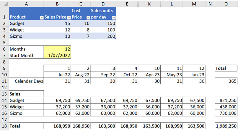
The beauty of dynamic arrays is that they automatically expand as required. If we add a new Gizmo product to the table at the top of sheet, the dynamic array formulas all automatically expand to include it. See Figure 2. 

In the past, the SUM solution was the missing piece of the total dynamic array solution. That has now been solved.

If we need to add even more products, we only need to insert extra blank rows below the table and within the budget section – a simple procedure.

The companion video will cover all the examples above, and I will share three custom functions to make the process even easier. There are companion files (start and end) with all the examples and formulas.

Neale Blackwood CPA runs A4 Accounting, providing Excel training, webinars and consulting services. Questions can be sent to [email protected]