Loading component...
At a glance
This is the first in a three-part series on Excel reporting using dynamic arrays, you can read part 2 and part 3 here.
Since their introduction in 2020, dynamic arrays and the functions associated with them have evolved. This article demonstrates some advanced dynamic array techniques that can be used to automate Excel reports.
The subscription version of Excel is required for these examples.
Why use dynamic arrays?
Standard Excel report formulas must be copied to other cells to populate ranges. If they are edited, the formula needs to be copied again.
A single dynamic array formula can automatically populate a vertical, horizontal or two-dimensional range.
This is called spilling, and it creates a spill range. The formula is only in the top left cell, which reduces the number of formulas that must be maintained.
Dynamic arrays can automatically expand to include new codes. In the past, new codes needed to be added to tables and reports. With dynamic arrays, adding a code to a table can automatically include the code in the report.
Worked example
This example combines various dynamic array functions to automate a report. The techniques are very powerful and flexible.
Consider reading the text and watching the video a few times to understand the concepts because they are new and different. Practice will also be required.
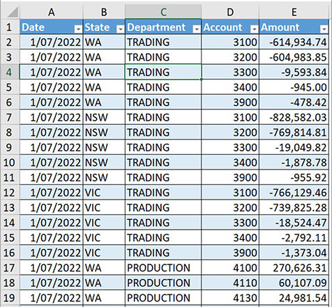
The data source for this example includes a General Ledger (GL) extract download with multiple years of data. This data has been defined as a formatted table named tblGLData – see Figure 1.
The actuals figures are up to January 2024.
Note: Only profit and loss accounts are included.
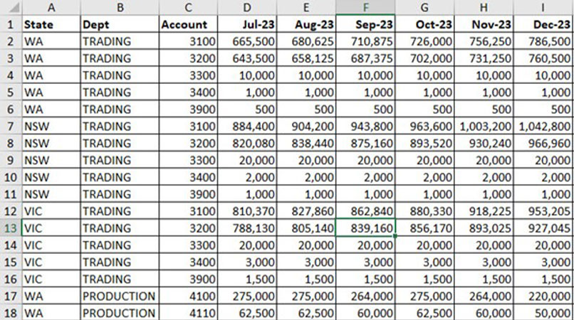
There is a standard budget structure with account details listed down the sheet and months going across the sheet – see Figure 2.
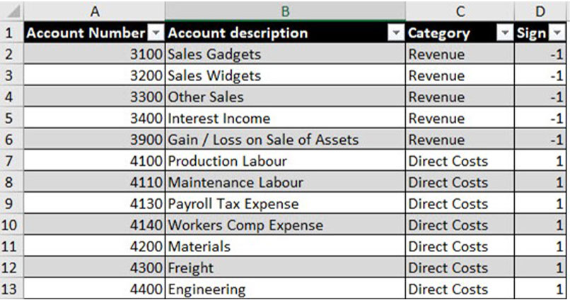
There is an account table that is also a formatted table named tblAccounts – see Figure 3.
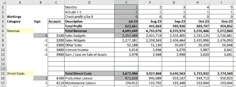
The report displays the monthly revenue and expenses across the page for a financial year. Actuals will be used if available. The remaining months will use the budget figures – see the report extract in Figure 4.
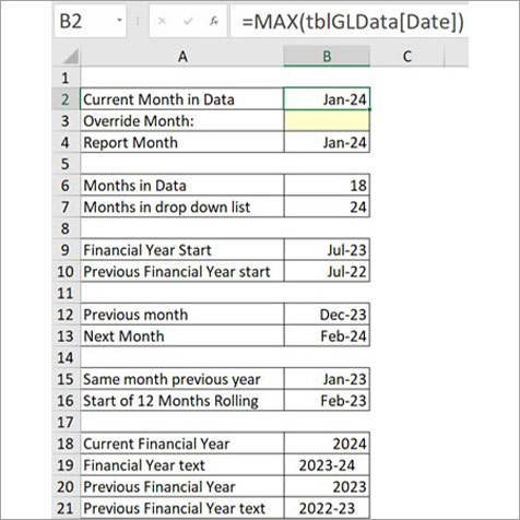
The Control sheet calculates several dates and other information – see Figure 5. Cells B4 and B9 are used by the report formulas.
Cell B2 determines the most recent date in the GL data table using the MAX function. The report month in cell B4 is used to calculate the other dates on the sheet.
The table in Figure 6 lists the formulas that are in the top left section of the report in Figure 4.

The formulas in Figure 6 are explained below and in the companion video.
Cell E1
=SEQUENCE(1,12)
This formula drives the whole report. It creates a horizontal spill range of 12 sequential numbers and determines how many columns to create. The number 12 is keyed in because the number of months will not change.
To refer to a spill range, use the top left cell reference of the spill range followed by the # symbol. To refer to the spill range in cell E1, use E1#.
The other formulas also spill to the right to match the cell E1 spill range. Cell D6 is the exception.
Cell E2
=(E4#<=Control!B4)*1
Cell B4 in the Control sheet has the current month for actuals. The above formula displays 1 if the month is an actuals month, and 0 if the month is a future budget month. The logical test will return either TRUE or FALSE. The result is enclosed in parentheses to enable multiplication.
Multiplying TRUE by 1 will return 1. Multiplying FALSE by 1 will return zero.
Cell E3
=IF(E2#=1,SUMIFS(tblGLData[Amount],tblGLData[Date],E$4#)+E5#,E5#-U5#)
This formula confirms the profit calculated in row 5 matches the data from the GL or the budget. The SUMIFS function calculates the actual profit by adding up the amount column when the date column matches the month.
Revenue is negative, so the profit returned is also negative. Hence, we add the calculated actual profit from row 5 to ensure it equals zero. The budget profit is calculated in cell U5 – see budget summary.
Cell E4
=EDATE(Control!B9,E1#-1)
This formula displays the column month. The starting month is determined on the Control sheet in cell B9.
Cell E5
=E6#-E15#-E33#
This formula calculates the profit by deducting the expenses from the revenue.
Cell D6
="Total "&A6
This formula is a standard formula that creates the total heading based on the input cell in A6. The & symbol joins text together.
Cell E6
=BYCOL(E7#,LAMBDA(x,SUM(x)))
Reporting Using Dynamic Arrays (Recorded webinar)
Ranges can spill down, so it is easiest to include totals at the top of spill ranges.
This formula adds up each column created by the two-dimensional spill range in cell E7. The BYCOL function provides each column to the LAMBDA function, which sums the column and spills across.
Cell B7
=CHOOSECOLS(SORT(FILTER(tblAccounts,tblAccounts[Category]=A6)),4,1,2)
This formula returns three columns from the tblAccounts table. The table is filtered using the FILTER function, based on the category entered in cell A6. The filtered rows are then sorted by the account column in the SORT function. The columns are then rearranged by the CHOOSECOLS function.
The 4,1,2 on the end means show the fourth column, followed by the first column, followed by the second column. This formula spills across and down to create a two-dimensional spill range of the revenue accounts.
The sign column is used to adjust the negative values for revenue codes. The GL data has negative values for credits. To display the revenue as a positive, the sign column is multiplied by the result of the SUMIFS function in cell E7.
Cell E7
=IF(E$2#=1,SUMIFS(tblGLData[Amount],tblGLData[Date],E$4#,tblGLData[Account],INDEX(B7#,,2))*
INDEX(B7#,,1),U7#)
This formula creates a two-dimensional spill range that returns either the actual month amount or the budget month amount.
It uses a SUMIFS function with formatted table references (called structured references) to summarise the actuals data based on the account number. The budget amount is calculated on the right-hand side in cell U7 – see budget summary.
The advanced parts of this formula are the two INDEX functions. The first refers to the second column (the account number column) of the two-dimensional spill range in cell B7. The second refers to the first column (the sign column) of the E7 spill range.
The number of rows that are populated by the formula in E7 will vary depending on the category used in the input cell A6.
The range B6:E7 can be copied and pasted into cell B15 to calculate the direct costs and cell B33 to calculate the indirect costs.
Totals
Rows 5, 6 and 7 all spill across and need to be totalled. Instead of three separate SUM formulas, a single SUM formula that spills down can add up all the rows in the three spill ranges – see Figure 7.
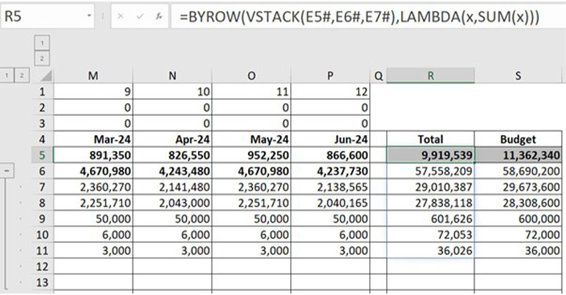
Cell R5
=BYROW(VSTACK(E5#,E6#,E7#),LAMBDA(x,SUM(x)))
This formula uses the VSTACK function to combine the three separate spill ranges into a single spill range. The BYROW function then takes that spill range and provides each row to a LAMBDA function to SUM them.
Cell R15
=BYROW(VSTACK(E15#,E16#),LAMBDA(x,SUM(x)))
This formula uses the same technique as cell R5 but for two spill ranges. This formula has been copied to cell R33.
Budget summary
The helper cells on the right of the report are used to summarise the budget based on the report structure. This simplifies the formula in cell E7 because it can link to the budget on the right rather than include another long formula for the budget.
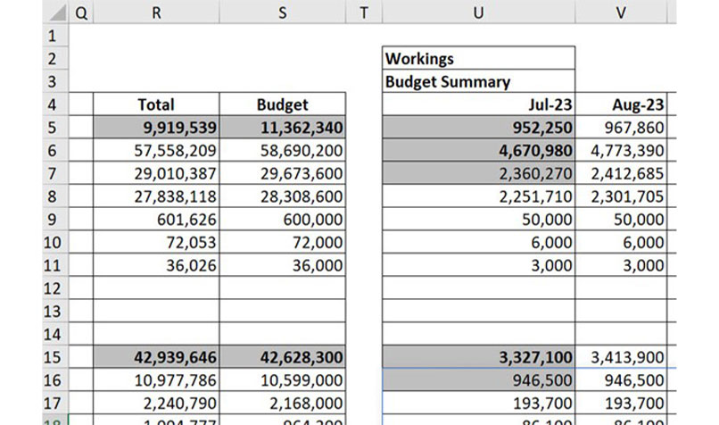
Cell U7
=SUMIFS(OFFSET('Budget Data'!C2:C175,,E$1#),'Budget Data'!C2:C$175,INDEX(B7#,,2))
This summarises each month’s figures from the Budget Data sheet. The budget structure used is not easy to extract from. The OFFSET function allows the range to sum (the first argument) in the SUMIFS function, to move across the sheet with the spill range.
The formula in cell U7 can be copied and pasted in cell U16 and cell U34 for the other two categories.
The profit formula in cell E5 can be copied to cell U5 for the budget.
The total monthly total from cell E6 can be copied to U6.
The total formulas from column R can be copied across to column AG to total the budget rows.
Column S has links to the total budget figures in column AG.
The budget section is shown in Figure 9.
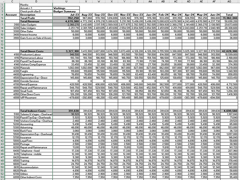
Automation
New accounts added to the tblAccounts table will be automatically inserted in the report. When the February data is added to the bottom of the table tblGLData, the report will automatically update to change the February month from budget figures to actual figures. The companion video shows this automatic monthly update.
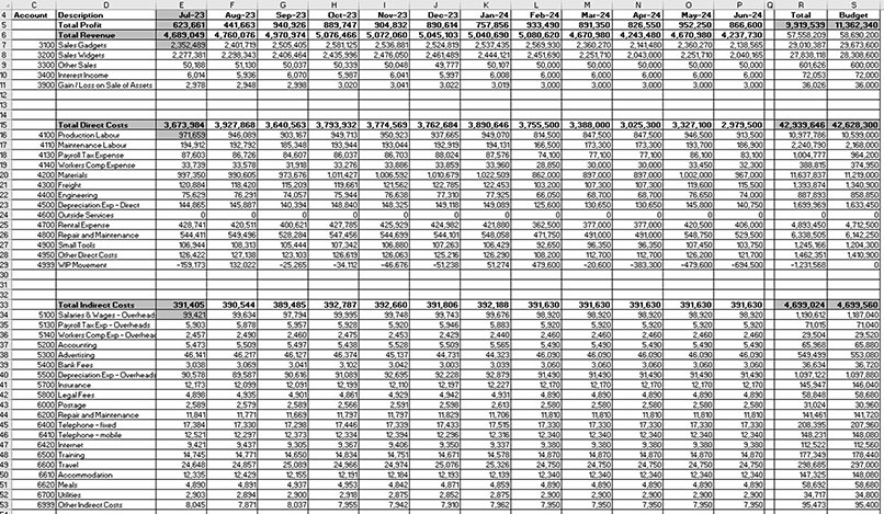
The final report is shown in Figure 10.
New mindset
Dynamic arrays require a different way of looking at formulas. Instead of cells, think in terms of ranges – whether horizontal, vertical or two-dimensional. Practice and trial and error will also be required.
Companion file
The companion file includes the report and data plus a version of the report using standard Excel formulas. You can download the example file to see all the formulas.

