Excel Tips: Automate reports with dynamic arrays – part 2

This is part 2 of a 3-part series. See part 1 and part 3 here.

Part 1 covered automating a 12-month reforecast report in Excel using dynamic arrays. Part 2 uses dynamic array formulas to automate a standard month and year-to-date (YTD) report with variances, including prior year comparisons. The data sources for Parts 1 and 2 are the same. This report also enables reporting by state.

General ledger

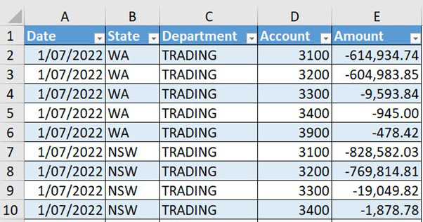
The general ledger (GL) data is shown in Figure 1. It contains multiple year data and only includes profit and loss accounts. It is in a formatted table called tblGLData.

Budget

The budget data sheet has a standard budget layout – see Figure 2. 

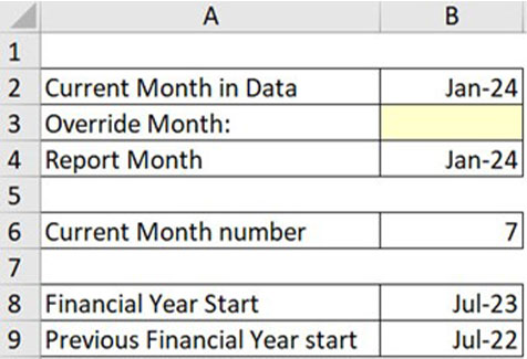
The Control sheet has the date information for the report – see Figure 3.

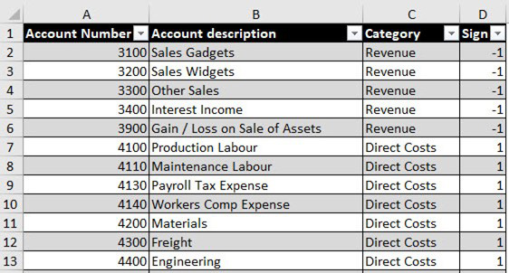
The GL accounts are in a formatted table called tblAccounts – see Figure 4.

The sign column is used to convert the negative revenue amounts in the GL data set to positive values for the report. The sign is also used in the variance calculations. 

Range names

Range names can shorten formulas that refer to formatted tables. Shorter formulas are easier to read, understand and maintain.

Range name rules

There are three main rules for creating range names.

1. They cannot start with a number.
2. They cannot contain a space (the underscore character and full stop are allowed).
3. They cannot be the same as a cell reference. Qtr1 may seem to be an acceptable name, but it is also a cell reference. Most two or three letter combinations are also column references. Qtr_1 is acceptable.

Range name prefixes

The range names prefixes are.

• acc – refers to columns in the tblAccount table.
• act – refers to columns in the tblGLData (actuals) table.
• bud – refers to columns in the Budget Data sheet.

Dynamic arrays and spilling

All the dynamic array formulas in this report spill down. This means the formula in the top cell populates the cells beneath, creating a spill range. The cells beneath must be empty, otherwise a #SPILL! error will display. To refer to a spill range, use the top left cell reference followed by the # symbol, e.g. A1#. 

Budget structure

Two additional columns are required in the budget structure to simplify the budget formulas in the Report sheet.

Column R in the budget data sheet lists the current month values. Column S has the current YTD values – see Figure 5. Note: The middle month columns have been hidden. 

Cell V1 is linked to the Control sheet and holds the current financial year month number.

The formula in cell R2 extracts the current month value and spills down the column to match the rows in the range reference. 

=INDEX(D2:O175,,V1)

This is an advanced use of the INDEX function. The first argument is the range to extract from. The second argument in the INDEX function is the row number to extract. If you omit the second argument, as in this formula, it returns the whole column from the range. 

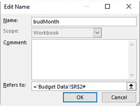
The third argument is the column number. In this case, the INDEX function extracts the seventh column from the range of monthly data. This spill range is named budMonth. 

Figure 6 shows the definition of the range name using the # symbol to refer to the spill range.

The formula in cell S2 that calculates the YTD amount is more complex. 

=BYROW(OFFSET(D2:D175,0,0,,V1),LAMBDA(x,SUM(x)))

It uses an OFFSET function to create a range that expands as the year progresses. It sums each row as it spills down.

OFFSET(D2:D175,0,0,,V1)

This OFFSET function has a starting range of D2:D175 (July column). It then offsets (moves) zero rows and zero columns from that starting range ,0,0 in the formula. The empty fourth argument instructs Excel to have the same number of rows as the starting range. The reference to cell V1 (7) means create a range that is seven columns wide including D2:D17. This is another advanced Excel technique.

The BYROW takes this range and splits it into separate rows and passes each row to the LAMBDA function as the variable x. The LAMBDA function uses the variable x in a SUM function to add up each separate row as it spills down. This spill range is named budYTD.

Report structure

The report structure is shown in Figure 7.

There are spare rows in each report section to enable the spill ranges to expand if new accounts are added. Inserting extra blank rows enables more accounts.

Selecting a state

There is a drop-down state selection in cell D3 of the Report sheet – see Figure 8.

The formula for cell E7 for the current month actuals is: 

=SUMIFS(actAmount,actState,$D$3,actDate,$E$2,actAccount,$C7#)*$B7# 

Each name starting with act represents a column in the tblGLData table. This SUMIFS function adds up the Amount column based on three conditions.

1. The state column matches the state selected in cell D3.
2. The date column matches the date in cell E2.
3. The account column matches the account in cell C7. 

Multiplying the result by cell B7# converts the negative revenue values from the GL table into positives for the report.. One formula can be used for both revenue and expense accounts.

Current month budget

The formula for cell F7 for the current budget month is:

=SUMIFS(budMonth,budState,$D$3,budAccount,C7#) 

Budget values are all entered as positive so no adjustment for sign is required. This SUMIFS has two conditions (State and Account), because the current month values are in the budMonth column.

YTD actuals 

The formula for cell J7 for the YTD actuals is: 

=SUMIFS(actAmount,actState,$D$3,actDate,”>=”&$E$1,actDate,”<=”&$E$2,actAccount,C7#)*B7# 

This is like the calculation in cell E7, but it uses two conditions on the date column to handle the start and end month. When using the greater than and less than symbols, they must be enclosed in quotation marks and joined to the condition using the & symbol. The & symbol joins text together.

YTD budget

The formula for cell K7 for the YTD budget is:

=SUMIFS(budYTD,budState,$D$3,budAccount,C7#) 

This is the same formula as the month budget, but it uses the budYTD range as the range to sum.

Variances

The calculation of variances is different for revenue and expenses. 

Favourable variances (shown as a positive value) for revenue require actuals to be above budget. Favourable variances (shown as a positive value) for expenses require actuals to be below budget. The sign column has -1 for revenue and 1 for expenses. The sign column enables a single variance formula for revenue and expense variances. 

The variance formula for cell G7 is: 

=(F7#-E7#)*$B7# 

This deducts actuals from the budget and multiplies the result by the sign value. 

Variance percentage

The variance percentage formula for cell H7 is:

=IF(F7#=0,0,G7#/ABS(F7#)) 

The IF function avoids the #DIV/0! error and displays zero if the budget is zero. The ABS function converts all numbers to positive by removing the negative sign. Using the ABS function ensures negatives are handled correctly.

Totals

The total formulas for the value columns all use the # symbol to refer to the spill range above. The formula for cell E16, which adds up the actual month revenue that starts in cell E7 is.

=SUM(E7#)

Other formulas

All the other formulas are either based on those explained previously or are standard Excel formulas.

Companion video and file

The companion video also demonstrates the following:

• adding next month’s data to automatically update the report
• techniques to handle hiding the blank report rows
• listing all the range names and their definitions.

 The companion file includes the report and data plus a version of the report using standard Excel formulas. You can download the example file to see all the formulas.