Excel tips: how to sort lists using dynamic arrays

Dynamic arrays are a new feature in Excel 365 (subscription version). The feature is being rolled out to all Excel 365 users in July 2020. Older versions will not receive this functionality.

SORT function

This new function allows you to dynamically sort a list using a formula. The list can be vertical (column-based) or horizontal (row-based). This function works well in combination with the UNIQUE and FILTER functions we explored last month.

SYNTAX

Note: when reading Excel’s formula syntax, any arguments within square brackets are optional. When omitted, their default value is used.
SORT(array,[sort_index],[sort_order],[by_col])

array – the range to sort. This can be a single or multi-column range. This can also be another function that returns a range, e.g. the new UNIQUE function covered last month.

sort_index – optional. This is a number that specifies the row or column number within the range to sort by. If omitted, 1 is used, meaning the first column is used to sort the range.

sort-order – optional. You can choose between ascending and descending. Use 1 for ascending and -1 for descending. If omitted, 1 (ascending) is used.

by_col – optional. This determines the direction of the sort. FALSE (default) sets the sort direction as rows (vertical range). TRUE sets the sort direction as columns (horizontal range). Since the default is used for a standard, vertical table-based range, you would omit this argument in most cases.

SORT function example

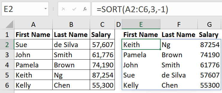
Figure 01 shows a table on the left and the sorted table on the right. The table on the right is sorted by the Salary column in descending order. A formula has been entered in cell E2 that creates the table on the right. 

The formula in cell E2 is

=SORT(A2:C6,3,-1)

The formula returns a range exactly the same size as the range it refers to – three columns wide and five rows long. The 3 means base the sort order on the third column (Salary). The -1 means sort in descending order.

Changing a value in the Salary column on the left could result in the order of the table on the right changing automatically.

SORTBY function

If the values you want to sort by are not in the range you want to return, you can use the SORTBY function. In our previous example, you may want to sort the list of names in order of salary, but not list the salary figure.

SORTBY(array,by_array1,[sort_order1],[by_array2],[sort_order2],…)

array – the range to sort. This can be a single or multi-column range. This can also be another function that returns a range, e.g. the new UNIQUE function covered last month.

by_array1 – first array is required, and the others are optional. This argument specifies the column number to sort by. You can specify more than one column.

If you do, it sorts by the by_arrays listed from left to right. sort order1 – optional. Each by_array argument can have its own sort order – 1 specifies ascending order and is the default, -1 specifies descending.

SORTBY function example

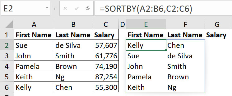
In Figure 02, I have used the SORTBY function in cell E2 to list the names only, sorted in ascending order based on salary. The formula in E2 in Figure 02 is

=SORTBY(A2:B6,C2:C6)

This first range is the range that will be sorted. It has two columns and five rows. The second range is the single column range (Salary), and this is used to determine the sort order. Because the third argument has been omitted, it has sorted the Salary column (C2:C6) in ascending (default) order.

Sequence function

This new function returns a list or table of sequential numbers. It can be used on its own or with other functions that require sequential numbers.

Syntax

SEQUENCE(rows,[columns],[start],[step])

rows – specifies how many rows to return. Although it is not listed as optional, you can omit this argument if you want a horizontal list of sequential numbers. If omitted, 1 is returned.

columns – optional. Specifies the number of columns to return. If omitted, 1 is used.

start – optional. Specifies the starting number for the sequence. If omitted, 1 is used. 

step – optional. Specifies the number to add to the sequence. This can be a fraction, and it can be negative. If omitted, 1 is used.

Sequence function example

Let’s say you need a loan calculator that handles a varying number of years. Normally this means building the schedule to handle all the years up to a maximum that you determine, say 30 years. This means you can’t handle 31 years without modifying the schedule. With SEQUENCE, you can create a totally flexible schedule that has no limit.

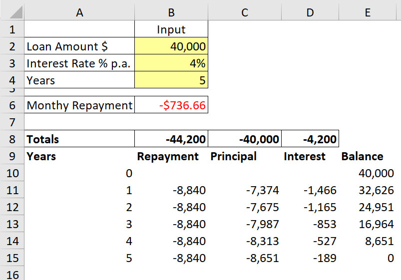
Figure 03 has a loan schedule for five years.

In the companion video, I will go into detail about all the formulas used in Figure 03 and Figure 04. Some of the formulas are complex, but the complexity is not due to the dynamic arrays. For this article, I will focus on a few of the formulas that explain how and why this technique works.

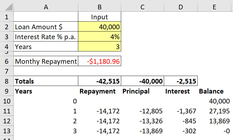
Changing cell B4 will automatically change how many years are displayed and calculated – see Figure 04.

The initial formula to create the schedule is in cell A10. It is

=SEQUENCE(B4+1,,0)

This creates a sequential list of numbers that is one more than the number in cell B4. The sequence starts at zero due to the zero at the end of the formula. In Figure 04, cell B4 has 3, so the SEQUENCE function creates a list of four numbers starting at zero. Zero in the list represents the starting balance.

The formula in cell A10 is a dynamic array. As per the first article I wrote in May, we can dynamically refer to this vertical range by using the # symbol.

The formula in cell B10 is

=IF(A10#>0,B6*12,"")

By using the # symbol after A10, we dynamically refer to the vertical range no matter how long it becomes. The formula in B10 will spill down to match the entries in column A.

If the number in column A is greater than zero, then the annual total repayment is calculated by multiplying the monthly repayment in cell B6 by 12. If the number is zero, a blank cell is returned. Two quotation marks used together specifies a blank cell.

The entries in cells C10, D10 and E10 all have a similar IF function to B10, but the calculations performed are much more complex than in cell B10. Because they also use the # symbol, they too spill down as far as required.

The totals in row 8 also use the # symbol. The formula in cell B8 is

=SUM(B10#)

This sums the range from B10 down as far down as the formula spills. The formula in cell B10 will spill as far as required to match the formula in cell A10.

The formula in cell B8 has been copied across for the other totals.

The reason the totals are at the top is that we don’t know where the end will be.

RANDARRAY function

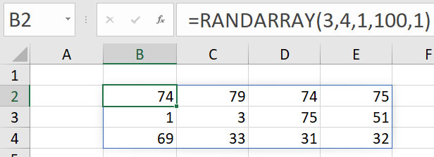
This function produces a range of random numbers. This can be useful for testing, training or forecasting, but has limited use in an accounting setting. More details of this function will be published on the INTHEBLACK website version of this article.

The companion video and Excel files (blank and complete) will go into more detail to demonstrate these techniques.

Neale Blackwood CPA runs A4 Accounting, providing Excel training, webinars and consulting services to organisations around Australia. Questions can be sent to [email protected]