Excel tips: how to use CONCAT and TEXT JOIN

Excel is known for its ability to handle numbers but it also has many functions dedicated to manipulating text. The latest release, Excel 2016, has added two functions that simplify joining text together.

In the past, there were two methods to join text and neither were scalable. The more text joins you required, the longer the formula. Figure 1 demonstrates the two techniques.

Both examples have a space between the two names. The CONCATENATE function separates the text to join with commas. The & symbol is like a connector and it, too, joins text together.

When you only need to combine two or three pieces of text together the & is easier to use and creates a shorter formula.

The new text functions in Excel 2016 are CONCAT and TEXTJOIN. Both accept a range, which means that they scale very easily. Extending the range can increase the length of the text string.

CONCAT is the simplest of the new functions. It only accepts a range and it joins all the text in that range together. This means you need to handle spaces or other joining characters within the cells in the range. Figure 2 has an example of the CONCAT function.

You can join multiple ranges together in CONCAT by separating the ranges with commas.

The TEXTJOIN function has two options. One lets you specify a separating character, for example, a space. The other lets you ignore blank cells.

Syntax:
TEXTJOIN(Delimiter, Ignore_Empty,Text1,[Text2]…)

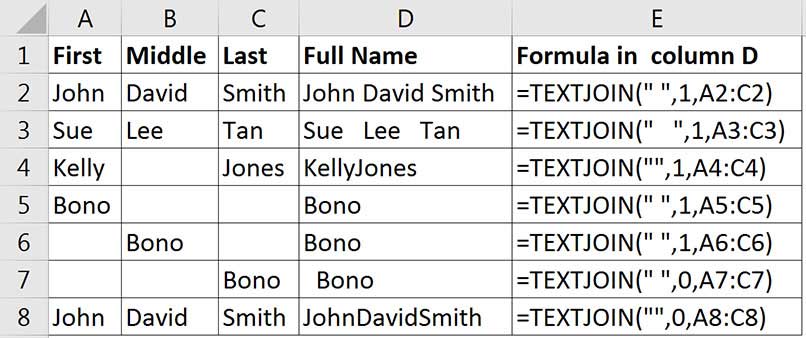
Delimiter – a text string to place between each cell’s text. Typically, this is a space. You must enclose the delimiter text in quotation marks, see examples in Figure 3. The delimiter can be more than one character.

Ignore_Empty – you enter TRUE to ignore empty cells and FALSE to include empty cells. You can use 1 for TRUE or 0 for FALSE. Using FALSE (0) works like CONCAT. See examples in Figure 3.

Text1, Text2 – this is the range that has the text to join. You can include multiple ranges separated by commas.

The formula in cell D3 in Figure 3 has three spaces as the delimiter.

The formula in cell D4 has a blank as the delimiter; two consecutive quotation marks represents a blank in Excel. This means nothing is inserted between the names.

Although rows 5 and 6 have only one name, cells D5 and D6 don’t have any extra spaces in them because the Ignore_Empty argument was set to 1 (TRUE).;

Cell D7 does have leading spaces because the Ignore_Empty argument was set to 0 (FALSE). In most cases, you would not use a delimiter and have 0 (FALSE) for the Ignore_Empty argument.

Cell D8 uses a blank delimiter and doesn’t ignore empty cells. This combination is redundant as it provides exactly the same result as using the CONCAT function, which is simpler to create.

Two practical applications of the TEXTJOIN function follow.

Creating sentences

Let’s say you use standard sentences when providing commentary for each month’s results. You could use IF functions to change certain words and then use the TEXTJOIN function to join all the words in a sentence.

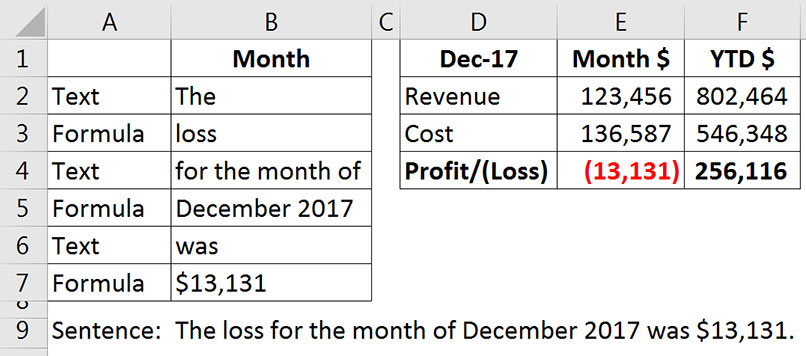
The example shown in Figure 4 has a simple report in D1:F4 which is the basis for the sentence in row 9. 

Column A describes the entry in column B. It is common to have the sequence Text, Formula, Text as many words will be fixed while other words will be variable or even optional.

The sentence formula in cell B9 is:
=TEXTJOIN(" ",1,B2:B7)&". "

This formula places a space between the entries and ignores empty cells.

Note: I use the & on the end of the TEXTJOIN function to correctly handle the full stop. If the full stop was in the text range, it would have had a space in front of it. There is also a space after the full stop in case you want to join sentences together.

The formulas in the B2:B7 range are:
Cell B3:
=IF(E4>=0,"profit","loss")

This simple IF function switches between the words profit or loss based on cell E4’s value.

Cell B5:
=TEXT(D1,"mmm yy")

When referring to dates in text you need to use the TEXT function to convert the date into a text date format. If you don’t, the date will appear as a meaningless number.

The TEXT function can be used to correctly display dates, numbers and percentages. The formats used must be enclosed in quotation marks and are based on the formats in the Custom section (last option) of the Number tab in the Format Cells dialog.

Cell B7:
=DOLLAR(ABS(E4),0)

I have used the ABS function on cell E4 to remove negatives. When describing the result for the month, the value displayed will always be positive. The number will be defined by the word profit or loss used earlier in the sentence.

When using numbers in text, the numbers will have no format unless you use either the TEXT function (as per cell B5) or the DOLLAR function. The DOLLAR function is designed to display numbers as currency. The 0 at the end of the formula defines the number of decimal places to display. To display other currencies you would need to use the TEXT function.

Creating codes

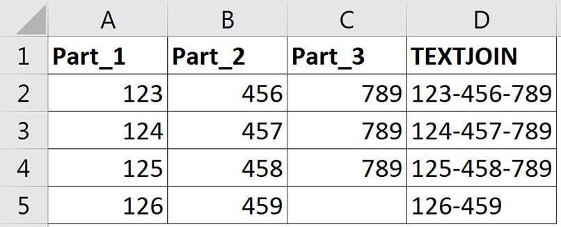
Some codes have structure built in to them. You might have three parts, with each part separated by a dash, or sometimes only two parts separated by a dash. Figure 5 shows the solution.

The formula in cell D2 is copied down; it is:
=TEXTJOIN("-",1,A2:C2)

This adds the dash between the codes and it ignores empty cells.

What function to use?

The CONCAT function is simple to use but the flexibility of the TEXTJOIN function provides more opportunities to automate the following:

• report headings
• journal narrations
• descriptive text
• code creation
• names and addresses
• instructions

Note: You could copy and paste, or even link the results of CONCAT or TEXTJOIN functions in Microsoft Word or PowerPoint.

The companion video and Excel file will go into more detail to demonstrate these techniques.

Neale Blackwood CPA runs A4 Accounting, providing Excel training, webinars and consulting services to organisations around Australia. Questions can be sent to [email protected]