Loading component...
At a glance
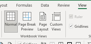
The standard grid view of Excel is called the Normal view. The other three icons in Figure 1 have specialised features that can make printing easier.
Page break preview icon
This view changes the Excel grid to show what will be printed (white background) and what won’t be printed (grey background) – see Figure 2. It also displays the page numbers as a watermark on the screen. This helps you understand the sequence of your printout.
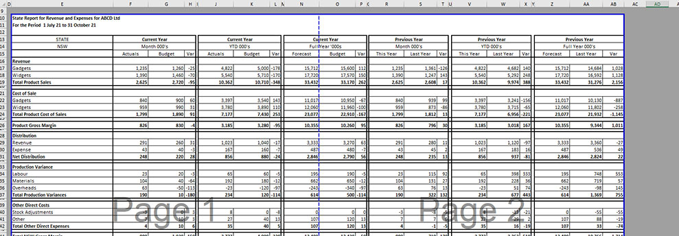
This view displays the print area and page breaks with solid blue lines. The dotted blue lines are where Excel estimates the pages will break based on the current print settings.
You can click and drag the dotted blue lines to move the page breaks. The dotted lines become solid lines when you move them.
Moving an automatic page break may also amend the zoom percentage being used in printing. Check the Page Layout ribbon tab (Figure 3) to see the Scale percentage.

Anything below 75 per cent tends to be difficult to read.
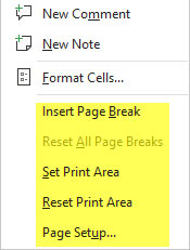
This view has extra print options when you right-click on the sheet – see Figure 4.
Page layout icon
This view makes Excel look like Word and provides the most accurate representation of how the pages will look printed out. Note that this view is not compatible with the Freeze Panes feature, also on the View ribbon.
Freeze Panes keeps rows at the top of the grid and columns to the left. If you have used Freeze Panes, a warning message is displayed before allowing you to proceed.
This view is ideal if you are creating headers or footers. You can click in the header or footer sections and a new ribbon will display with all the available options – see Figure 5.
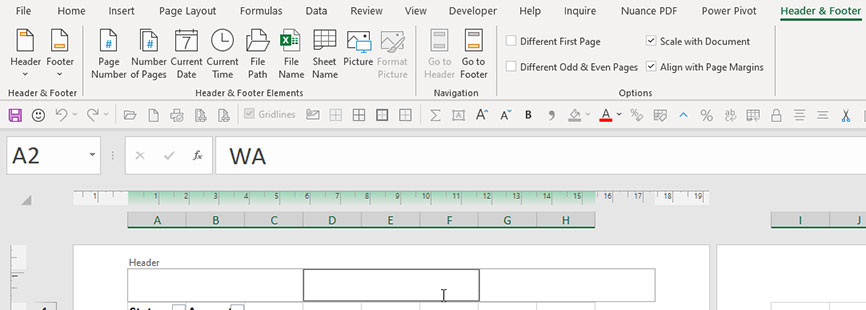
The default display on this view is to show the margins on the pages. You can click the icon between the pages to hide the margins.
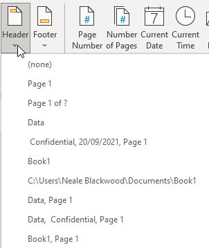
The two icons on the left of the ribbon offer standard header and footer entries via a dropdown – see Figure 6.
Small icons
At the bottom right-hand corner of the Excel screen (to the left of the zoom percentage) are three small icons for the three different views. The sequence of the icons from right to left is Normal, Page Layout and Page Break Preview – see Figure 7.

Custom views icon
The idea behind the Custom Views feature is that you can capture the following display and print settings at a point in time, including hidden rows or columns in all the sheets, print settings in all the sheets and hidden/visible sheets. You can then reinstate all the settings you captured by selecting a specific custom view.
For all its possibilities, custom views also has some limitations.
You cannot use custom views if you have a formatted table in the file. Adding a formatted table to a file with custom views will disable access or use of custom views.
A custom view captures hidden rows at the time it is created. If you use a filter to hide or unhide rows and the data changes, then the visible and hidden rows captured by a custom view may no longer be valid.
Custom views are useful for capturing which sheets are hidden and which are visible at a point in time, and a custom view can quickly reinstate the hidden and visible sheets. The limitation is that sheets added after the custom view is created will not be included in the custom view settings.
Custom views cannot be edited. If changes are introduced after a custom view has been created, you will need to delete the old custom view and then re-create it to handle the new structures. Custom views are easy to create and use. If your file structure doesn’t change much, custom views can be useful.
Their limitations do reduce their practical long-term use in many cases. The companion video to this article will take you through creating and using a custom view.
Unhiding sheets
In the most recent versions of Excel, you can unhide multiple sheets by right-clicking a sheet tab and choosing Unhide.
You can use the Shift key or the Ctrl key to select multiple sheets to unhide, then click OK. In the older versions, you can only unhide one sheet at a time and custom views may be the best option to speed up unhiding/hiding multiple sheets in one step.
Excel printing tips
Set your print area (Page Layout ribbon) to limit and control what range will be printed.
Always check the Print screen (File tab) before printing for the first time. Check the number of pages and the page breaks.
Use the built-in options on the Print screen (File tab) to save some time.
Some useful options are
Orientation – Portrait or Landscape
Custom Margins – there is a Narrow option
Scaling – Fit Sheet to One Page – Fit All Columns on One Page
Neale Blackwood CPA runs A4 Accounting, providing Excel training, webinars and consulting services. Questions can be sent to [email protected]

