Excel Tips: Under-used Excel features

It’s natural to focus on Excel’s new features, but there are a lot of existing features that are under used. Here are a few that can make your work life much easier.

Excel Windows

This refers to the ability to show the same file on separate screens. This feature was added many versions ago, but many people are not aware how useful it is. 

Most modern workstations have at least two screens. It is possible for the same file to be displayed in a second window on a separate screen, or two or more separate sheets from the same file can be visible at the same time. 

Each window has its own ribbon and Quick Access Toolbar. This makes copying between the sheets much easier.

The View ribbon tab has the Window options — see Figure 1.

Each click of the New Window icon creates a new window of the current file. The Arrange All icon will arrange the open windows on the one screen, which is handy if you have a very large screen. 

Each window has a number on the end of the file name in the title (Figure 2). See the Warnings below which explain why these numbers are important.

Warning: I recommend closing all the windows labelled 2 or higher before saving and closing the file. There are two reasons for this.

1. The new windows (2 and higher) have no view or print settings. The number 1 window has all the existing view and print settings. If you close the number 1 window and then save and close the file, all the existing view and print settings are lost and must be reset. You need to close windows numbered 2 and above before saving and closing the file.
2. If you save and close the file with multiple windows open, then those extra windows will be visible when the file is opened. This could be confusing for a first-time user or someone opening the file on a laptop.

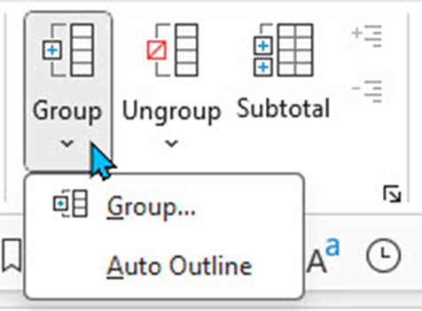
Being able to quickly hide and unhide rows and columns saves time. The grouping icons on the Data ribbon tab (Figure 3) make this easy to implement. 

Grouping has the added advantage of displaying icons to show that there are hidden rows/columns — see Figure 4.

The grouping keyboard shortcuts are:

Apply grouping - Shift + Alt + right arrow. 

Remove grouping - Shift + Alt + left arrow.

Automated grouping

Excel can use the structure in an existing report to automatically apply grouping. Excel bases the grouping on the formulas in the report. Select a cell in the report and use the Auto Outline option shown in Figure 3. Figure 5 has a before and after example.

Warning: Auto Outline cannot be undone. The grouping must be manually removed.

Grouping icon placement hack

Most of the time, the grouping icons work best at the bottom or to the right of the grouped rows/columns — see Figure 5. It is possible to show the grouping icons at the top and to the left. The option to change the position is hidden away.

Warning: Auto Outline cannot be undone. The grouping must be manually removed.

Grouping icon placement hack

Most of the time, the grouping icons work best at the bottom or to the right of the grouped rows/columns — see Figure 5. It is possible to show the grouping icons at the top and to the left. The option to change the position is hidden away.

In the Data ribbon tab, click the little arrow in the bottom right of the Outline section — see Figure 6. Untick the relevant options and click OK.

This positioning change applies to the whole sheet. It does not impact other sheets.

Figure 7 shows the revised icon placement using Auto Outline.

Automatic subtotals

Excel can automatically insert SUBTOTAL functions into a list. The Subtotal icon in Figure 3 enables you to automatically insert SUBTOTAL functions into a sorted list.

The list needs to be sorted by one of the columns. Select the list and click the Subtotal icon. Figure 8 has a list sorted by region (column A) plus the Subtotal dialog settings that will insert the SUBTOTAL function.

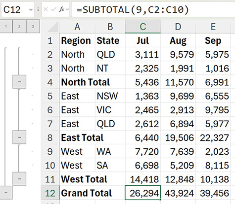
The first drop down in Figure 8 selects which column is sorted.

The second drop down chooses the calculation. It is usually Sum. Each column to be subtotalled is ticked. Figure 9 shows the result.

Note the grouping icons are automatically added. This makes hiding the detail rows easy — see Figure 10.

 

Making the subtotal values bold to match the text is a common request. The companion video demonstrates how to do that.

Note: The Subtotal dialog (Figure 8) has a Remove All button if required.

Note: You can’t use this feature with a formatted table. 

Visible cells

There are at least three ways to hide cells. Filtering, Grouping (examples above) and manually hiding rows or columns. Copying and pasting ranges with hidden cells can vary depending on how the cells were hidden.

When you copy a range in a filtered list, you are only copying the visible cells. Only the visible cells will be pasted.

If cells are hidden with Grouping or Hiding, then when you copy them, you are copying all the cells hidden and visible. When you paste, all the hidden content is also pasted.

Visible cells only

There is a technique to copy only the visible cells, no matter how the cells are hidden.

1. Select the range involved.
2. Press Alt + ; (Alt and the semi-colon). This selects the visible cells only.
3. Press Ctrl + C to copy.
4. Press Ctrl + V to paste.

Note: Only values are pasted after Visible Cells Only is used to copy. No formulas are pasted.

Custom lists

Dragging a cell with Jan will populate Feb and Mar. This is a built-in custom list of months. Excel has several date-based built-in lists, but you can also create your own custom lists.
This can be useful for departments, categories, people’s names or states.

To create a custom list, follow these steps.

1. Enter the list in a range and select it.

2. Press Alt F T in sequence, which opens the Excel Options dialog.

3. Click the Advanced option on the left.

4. Scroll to the bottom and click the Edit Custom Lists button — see Figure 11.

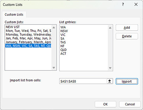
5. In the dialog that opens, click the Import button and click OK (Figure 12), then OK again.

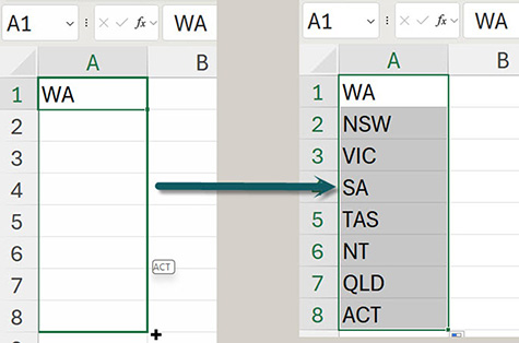
With the first entry in a cell, you can use the fill handle to drag the cell to populate the rest of the list — see Figure 13. Dragging will work for any item in the list.

Note: Custom lists are saved to your computer, not the file. If you have a laptop and a desktop, you must create the list on both to be able to use it on both. 

Sorting

A custom list can also be used to sort data. This is demonstrated in the companion video.

Language change

You can also change the default language for Excel’s controls like icons and buttons. For example, if changing from US to UK English, this changes “Customize the Ribbon” to “Customise the Ribbon”, and “Center” becomes “Centre”.

Note: Your organisation’s security settings may affect your ability to change this.

To make this change, follow these steps.

1. Click the File ribbon tab.
2. Click Options (bottom left).
3. Select the Language option.
4. In the Top section, click the Add a Language button.
5. Find and select your preferred language, in this example, English (United Kingdom).
6. Make sure the Set as Office display language is ticked at the bottom.
7. Click the Install button and then click OK.
8. Click OK.

Even though I advise against using the Merge and Centre format, at least it will be spelled correctly — see Figure 14.

The companion video and Excel file go into more detail to demonstrate these techniques.