Excel tips: how to use icons in your spreadsheets

When creating reports and dashboards, it is common to use icons to draw attention to results that require action. When deciding which icons to use, keep in mind that about 8 per cent of men and 1 per cent of women have some form of colour blindness. Red and green colour blindness is the most common. Therefore, using only colour to emphasise certain results may not always be effective. 

Excel has a built-in conditional format that allows you to automatically display icons based on cell values. The problem is that the default settings do not always show the icons you expect. 

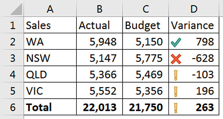
Adding an extra column with a formula can improve how the icons display. As an example of the defaults, examine Figure 1.

You can see here that the exclamation marks are shown next to negative as well as positive variances. The reason is that the default settings assume that the values in the range are indicative of the values you want to review. This means outliers can skew the calculation that determines which icons are displayed. Because the first two rows have large variances – both favourable and unfavourable – it causes variances in the middle to be treated the same.

It is much more reliable to create a formula to apply icons, which also allows you to build in parameters and tolerances. For example, you might have a tolerance of 5 per cent such that if a value is within 5 per cent of the budget, no investigation is required and no icon is displayed. Results outside of the 5 per cent tolerance may require further investigation and should display an icon.

How many icons?

When designing reports keep in mind that the more different icons you use the longer it takes to understand the report. Consider which actions you are expecting the reader of the report to take. In many cases, reports identify problems so that people can act on them quickly.

If your focus is on fixing problems, you only need one icon. If you also want to highlight exceptional results, you could use two icons. Showing an icon for achieving budget is probably a waste of an icon.

Worked example

Let’s expand on the tolerance example. We could have the following rules:

• Display a cross icon if sales are less than 95 per cent of budget
• Display no icon if sales are between 95 per cent of budget and 115 per cent of budget
• Display a tick icon if sales are greater than 115 per cent of budget.

These rules will identify if sales are slipping below budget and if a state has achieved an excellent result. Exceptional results should also be followed up, as they may offer ideas to improve overall sales.

To apply the rules, you need to use formulas to control the icons that display. We will add a column to the table plus two input cells to hold the 95 per cent and 115 per cent values. The revised report is shown in Figure 2. The input cells allow us to easily change rule parameters and hence control the icons.

The formula in cell E2, which has been copied down is: 
=IF(B2/C2<$H$2,-1,IF(B2/C2>$H$3,1,0))

The first IF function determines if the result is below the lower limit. In this case, -1 is displayed. The second IF function determines if the result is above the upper limit. In this case, 1 is displayed. If neither condition is met, a zero is displayed.

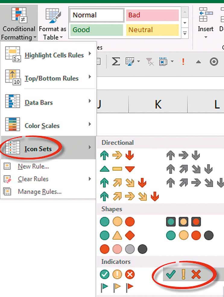
The values in column E are easier to use to control the conditional format icons. We can apply the same conditional format to E2:E6 as in D2:D6 and it will look the same, but we will edit the rule and amend the default settings. Select the range E2:E6 and on the Home ribbon click the Conditional Formatting icon and choose Icon Sets and the tick, exclamation mark and cross icon set as shown in Figure 3.

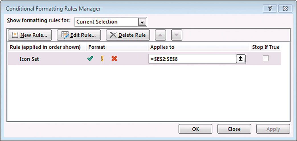
With the range still selected, click the Conditional Formatting icon drop-down and choose Manage Rules (the last option). This opens the Conditional Formatting Rules Manager (see Figure 4). The rule we created is listed. You can double-click the rule to edit it.

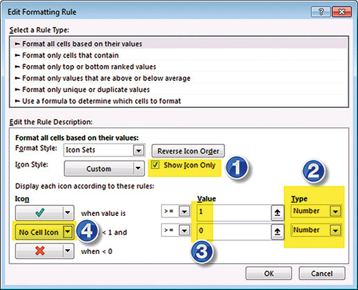
The icon sets rules are easy to control because we only have three possible numbers. We need to make the following changes highlighted in yellow and numbered in Figure 5:

1. Tick the Show Icon Only option – this will hide the numbers in column E.
2. In the Type drop-downs on the right change both to Number.
3. Enter 1 in the top Value box and 0 in the bottom Value box.
4. Click the middle icon drop-down and choose No Cell Icon (top of drop-down).

Click OK and OK again to apply the format.

The revised format is shown in Figure 6.

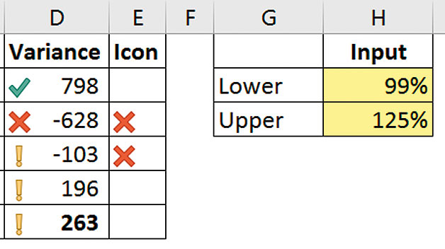
In Figure 7, I have amended the tolerances to demonstrate the effect on the report. The IF function works well for two or three icons. If you want to use more icons, you would use a table and the VLOOKUP function.

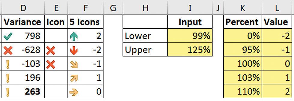
Figure 8 has a five-icon example.

The formula in cell F2 which has been copied down is: 
=VLOOKUP(B2/C2,$K$2:$L$6,2)

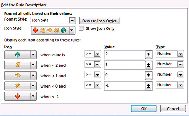
This looks up the percentage in the table and returns a number that we can then use in the Conditional Format rule shown in Figure 9. I have left the values visible in column F, so you can see the relationship of the number and the icon. The companion video to this article will include a more detailed explanation of this formula.

Error handling

If a budget value was zero, then errors may be encountered in both formulas. The following amended formulas handle errors. Cell E2:
=IFERROR(IF(B2/C2<$I$2,-1,IF(B2/C2>$I$3,1,0)),"")

Cell F2:
=IFERROR(VLOOKUP(B2/C2,$K$2:$L$6,2),"")

The IFERROR function allows you to specify an action if an error is encountered in a formula. In this case it will display a blank cell. The double quotation marks represent a blank cell. A blank cell won’t display an icon.

The companion video and Excel file will go into more detail to demonstrate these techniques.

Neale Blackwood CPA runs A4 Accounting, providing Excel training, webinars and consulting services to organisations around Australia. Questions can be sent to [email protected]