Loading component...
At a glance
Excel continues to be regularly updated and improved. Here are seven recent updates and how they can be utilised.
1. TRIMRANGE functionality
This is a major upgrade to the way ranges are referred to in Excel. The TRIMRANGE function has new range functionality. There is also a new range reference syntax that applies this functionality.
One of the problems with referring to ranges has been including extra data that has been added below an existing range. Formatted tables offered one solution to this problem, as the tables automatically expand to include extra data.
TRIMRANGE syntax offers another solution to this problem.
Ignoring the use of $ signs at this stage, the standard range reference syntax is A1:A10000.
The new range syntaxes use the full stop on either side of the colon to control a flexible start and/or end cell. There are three types:
A1.:.A10000 — This uses the first non-empty cell in the range as the first cell and the last non-empty cell as the last cell of the range. Flexible start and end cells.
A1.:A10000 — This uses the first non-empty cell in the range as the first cell and cell A10000 as the last cell of the range. Flexible start cell with a static end cell.
A1:.A10000 — This range starts with cell A1 and the last non-empty cell is the end of the range. Static start cell with a flexible end cell. I see this being the most popular usage of this new range referencing. It allows a long range to be defined to handle future data expansion. Data added to the end of existing data will be included.
Figure 1 shows these syntaxes using a small range to demonstrate. Each range formula in row 1 spills down.
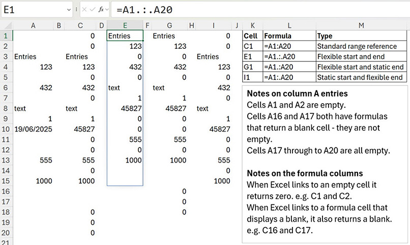
Note: In Figure 1, the spill range from cell E1 spills past the 1000 entry (cells E14 and E15) because cells A16 and A17 have formulas that return a blank cell, are not empty and are included in the E1 spill range.
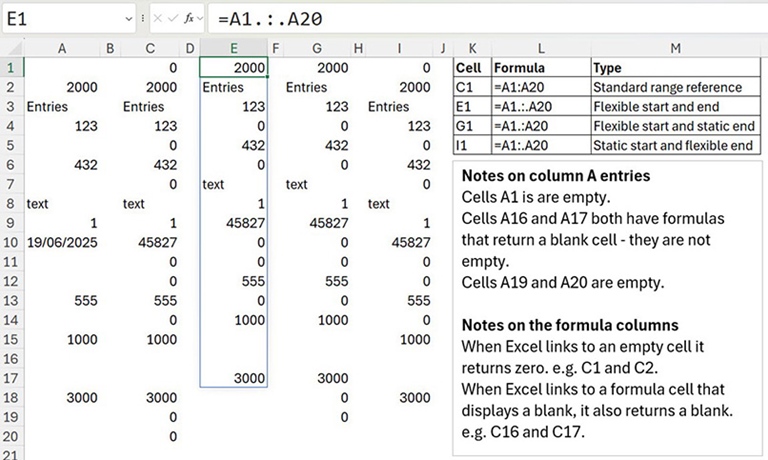
Figure 2 shows how the flexible ranges adjust when new data is added in cells A2 and A18.
The $ symbol can still be added to fix the row and column references, so they don’t change when copied.
E.g. $A$1.:.$A$10000
2. TRANSLATE function
The new TRANSLATE function can make life a bit easier when working with other languages in Excel.
The companion file has a list of languages and the codes used for converting between languages.
Note: This function requires an internet connection and there is a daily usage quota involved. The output may be blocked if used too frequently.
Worked example
Figure 3 shows different examples of this new function using one, two and three arguments.
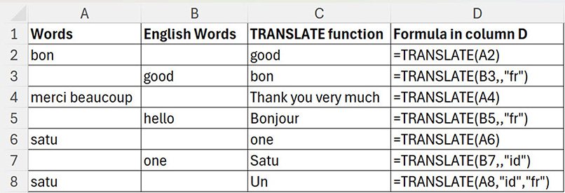
The first argument is the word or sentence to translate.
The second argument is optional and is the source language code. Excel will guess if this is omitted.
The third argument is the destination language code. This defaults to system language if omitted.
The language codes enclosed in quotation marks are fr for French and id for Indonesian.
3. PivotTable formats
One frustration with PivotTables is that there was no format applied to the values in the report. This required a manual change to the number format each time a report was created.
A recent update ensures the number format applied to the source data values will automatically flow through to the PivotTable report.
Note: Changing the source data number format after making the PivotTable won’t change the format for any existing PivotTables. It will update all new PivotTables created.
4. BYROW and BYCOL functions
These two functions allow spill ranges to be split into rows or columns and then have calculations performed on those rows or columns. When they were first implemented, they required the LAMBDA function to work.
They have now been updated to a simpler syntax. Excel’s standard functions like SUM and AVERAGE can be used. The LAMBDA function can still be used for more complex calculations.
Worked example
In Figure 4, I have created a two-dimensional spill range in cell C3 using the SEQUENCE function.
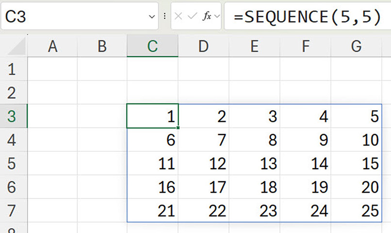
To add up the rows and columns, use the BYROW and BYCOL functions.
The left image in Figure 5 shows the old BYROW function syntax in the Formula Bar for cell B3. The right image shows the new syntax for the BYROW function.

It is much simpler. The same syntax change applies to BYCOL.
5. In-cell drop-downs
In-cell drop-downs have finally been updated in the desktop version of Excel. Typing a letter will reduce the entries in the list. Also, if the list range has duplicates, only the unique entries will be listed in the drop-down.
Worked example
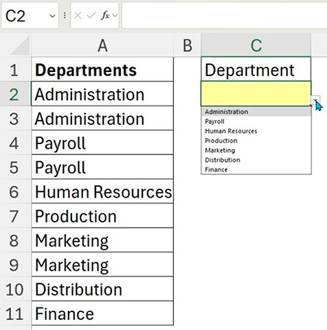
The list of departments in column A is used to create a drop-down list in cell C2.
Note: There are duplicate entries in column A. As you can see in Figure 6, the drop-down does not show the duplicates.
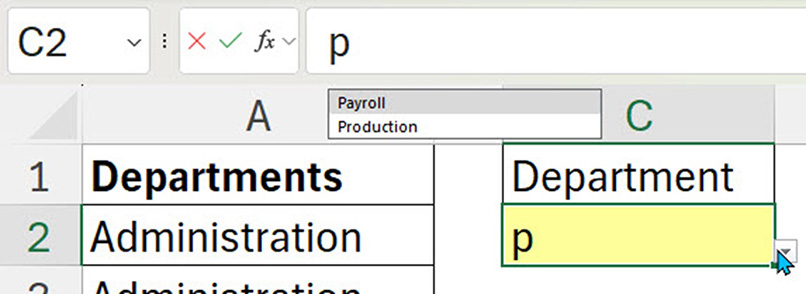
Typing a letter after selecting the drop-down list reduces the list — see entries under the Formula Bar in Figure 7.
6. Images in cell
Images can now be copied and stored inside a cell. This means they can be kept in tables, looked up and returned using formulas.
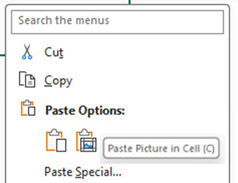
After copying an image, right click on the cell and choose the last paste icon — Paste Picture in Cell. See Figure 8.
Worked example
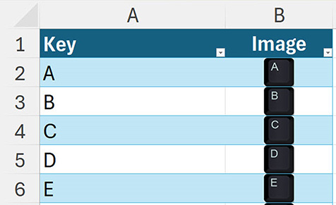
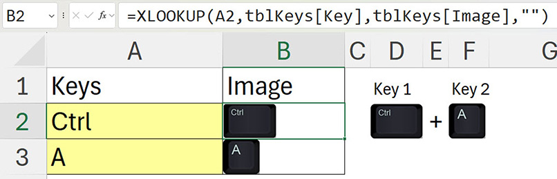
The companion file has a table (Figure 9) with keyboard images entered using Paste Picture in Cell. The table is named tblKeys.
Figure 10 shows how the XLOOKUP function can be used in cell B2 to extract the image based on the key name.
7. Focus Cell
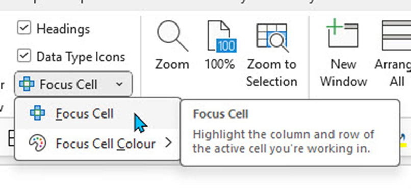
Do you work with wide or large spreadsheets? This update, called the Focus Cell, may make your day. A new feature in the View ribbon (see Figure 11) highlights the current row and current column of the active cell.
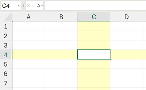
As the active cell moves, the row and column highlighting updates. See Figure 12.
A note on REGEX functions
Look out for three new functions call “regular expression” (REGEX) functions. They all start with REGEX. They allow searches and lookups based on patterns within codes. There are three REGEX functions. REGEXTEST, REGEXEXTRACT and REGEXREPLACE. If you don’t have them already, they’ll be coming soon.
The companion video and Excel file will go into more detail to demonstrate these updates.