Excel Tips: 2 DIY functions that use LAMBDA

Excel has a built-in technique to create custom functions. These DIY functions are created using a range name with the LAMBDA function.

This article will look at two custom functions that can help with accounting calculations:

• summing spill ranges
• handling financial years, months and quarters.

The techniques covered require the subscription version of Excel and use dynamic arrays.

The companion video provides more information about the techniques demonstrated. 

Naming convention

I recommend using a naming convention for all custom functions to help differentiate them from Excel’s built-in functions, I use the fn prefix, and I have also seen the fx prefix used.

Formula Bar Line breaks

The LAMBDA functions that follow are displayed in the Formula Bar. They are displayed using line breaks between the parts of the function. The line breaks make it easier to read and understand the formula.

When editing in the Formula Bar press Alt + Enter to insert a line break – see Figure 1. 

Excel has a keyboard shortcut to expand or minimise the height of the Formula Bar to show all the lines. 

Ctrl + Shift + U toggles the Formula Bar between a single line and multiple lines – see Figure 2. 

fnSUMDA custom function

This custom function adds up the rows or columns in a dynamic array spill range. The function requires two inputs: 

• the spill range or range reference to sum
• the direction of the sum (“r” for rows or “c” for columns). 

In Figure 3, the yellow cells enable the selection of a start date (B1), number of months (B2) and a department (A10). A report is generated based on the selections. The report spills across and down. SUMIFS function in cell D10 spills across and down to populate the report’s values. The D10 spill range must be totalled for rows and columns.

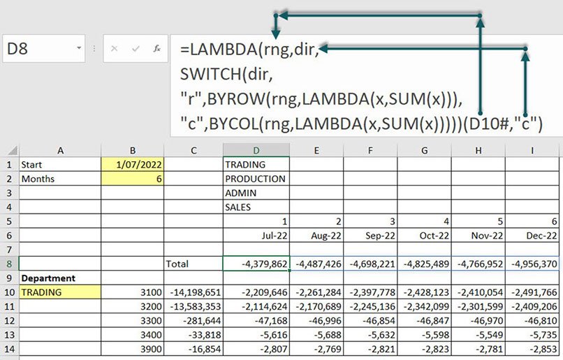
The test formula for the LAMBDA custom function formula is in cell D8.

The extra parentheses on the end enclose the test arguments for the LAMBDA formula. The spill reference D10# is passed to the rng argument. The “c” entry is passed to the dir argument.

The SWITCH function is new. It creates a self-contained lookup table in a formula. In this case, it defines the different calculations for the “r” and “c“ option for the dir argument. It also uses BYROW and BYCOL functions. 

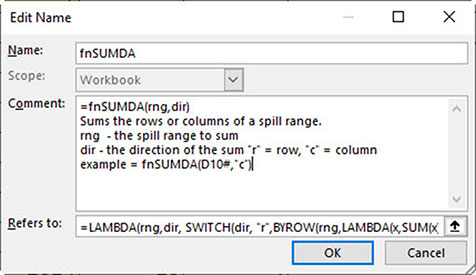
The Edit Name dialog for the fnSUMDA custom function is shown in Figure 4. To create a range name, use the Define Name icon on the Formulas tab.

The “Refers to:” section contains the LAMBDA formula without the extra set of parentheses on the end.

The “Comment:” section is free form text and is used to describe and explain the function. The description displays whenever you type the function name in the Formula Bar – see Figure 5. Completing this section is optional, but is recommended so other users can understand how the custom function works. 

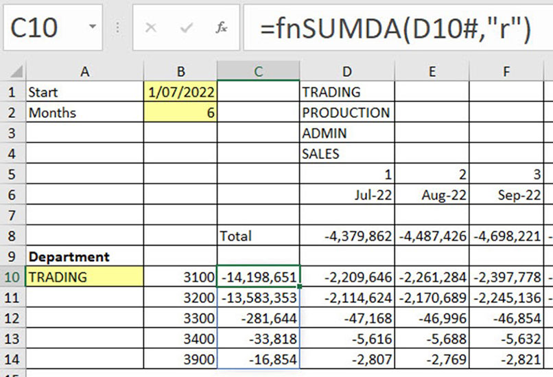
The fnSUMDA custom function is used in cell C10 – see Figure 6. The formula spills down to match the spill range.

fnFY custom function

Australia’s financial year offers challenges when working with years, month numbers and quarters. This custom function simplifies those calculations. It is also flexible enough to work with other financial years that start on 1 April or 1 October.

This function requires three arguments:

• the date to convert
• the starting calendar month number of the financial year
• the period value to return. 

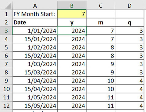
Figure 7 shows the structure. Figure 8 shows the LAMBDA custom function test formula in cell B3. The test formula has been copied across and down.

The LET function allows the use of variables within a formula.

The $A15 date is passed to the ref argument. The $B$1 value of 7 is passed to the start argument and B$2 entry of “y” is passed to the per argument.

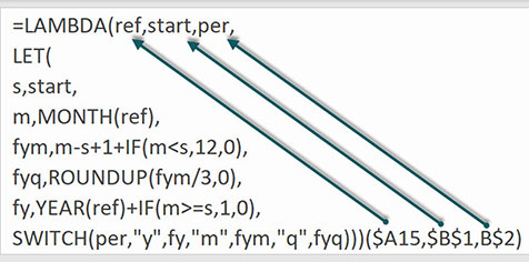
The start argument value from the LAMBDA function is passed to the s variable in the LET function. 

The ref date argument in the LAMBDA function is used in a MONTH function to calculate the calendar month number of the date that is captured in the m variable.

The calculation for the financial year month (fym variable) deducts the start month number from the calendar month number and adds 1. If the calendar month number is less than the start month, the number 12 is added. 

The financial year quarter (fyq variable) uses the ROUNDUP function with the fym value to calculate the quarter number. 

The financial year (fy variable) adds 1 to the calendar year if the calendar month is greater than or equal to the start month.

The SWITCH function defines what to return, based on the three options for the per argument from the LAMBDA function. The “y” option returns the fy variable value from the LET function.

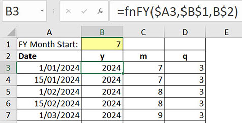
Figure 9 shows the fnFY custom function in cell B3. The formula has been copied across and down.

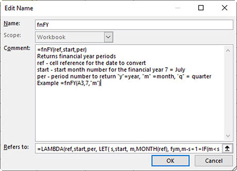
The Edit Name dialog for the fnFY custom function is shown in Figure 10.

If you copy a formula containing a custom function to another file, the custom function is copied across as well. 

Custom functions can be used to simplify complex calculations and create reusable solutions to difficult problems across multiple files.