Excel Tips: Formula cheat sheet

This is part one of a two-part series. Check out part 2 here.

Formulas are the building blocks of Excel. Formulas allow users to summarise huge amounts of data into manageable parts. Users can also build in decision-making and automate many tedious tasks using formulas.

The terms “formula” and “function” are often used interchangeably. While a function is a formula, not all formulas include a function. Functions are a subset of formulas.

When creating formulas, there are several techniques that can be used to speed up the creation and editing process.

It is a good idea to use the Formula Bar to do all formula work. The Formula Bar is located above the column letters and goes across the screen – see Figure 1.

While a formula can be created and edited in a cell, there are display limitations. The Formula Bar is easier to work in, especially for longer formulas. Use the End, Home and left and right arrow keys to move around the Formula Bar.  

Start a formula with +

All Excel formulas must start with the equals sign. However, it is not necessary to type the equals sign – pressing the plus sign will also start a formula. Excel will automatically insert the equals sign when the user presses Enter. 

Starting formulas with the plus sign can be more convenient because of the large plus sign key on the number pad at the far right of a full-size keyboard. This key is easier to use than the equals sign, which is tucked away in the middle of the keyboard on a PC.

For users who prefer to use a mouse, an equals sign button can be added to the Quick Access Toolbar. Click to insert the equals sign and continue to use the mouse to insert cell references and ranges.

Parentheses (brackets)

These symbols ( ) are called parentheses. When working with Excel formulas, they are often referred to as brackets. Brackets is the term used here.

Functions

The SUM function is Excel’s most-used function. It has its own icon and keyboard shortcut, making it easy to enter. The Tab key can be useful when using other functions.

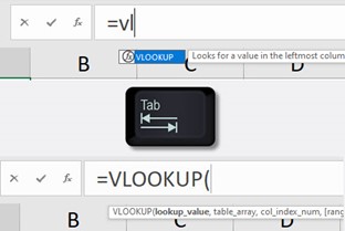
Type =vl into a cell to see Excel’s Intellisense feature in action – see Figure 2. 

There is only one function that starts with VL. When the function name is highlighted in blue, as in Figure 2, press the Tab key to insert it. This also inserts the opening bracket. 

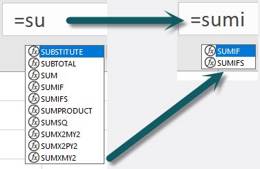
Depending on the letters typed – such as =su – a long list may appear. Use the up and down arrow keys to select a function, then press the Tab key. It is also possible to double-click a function name in the list with the mouse. As more keys are used, the list will filter and become shorter – see Figure 3.

This list can also include table names and range names that are being used in the file. This technique reduces the typing required to create formulas and reduces typing errors. 

Function arguments

The parts or sections of a function are called arguments. They are enclosed by brackets and separated by commas. A few functions do not require an argument, such as the TODAY function. Many functions have optional arguments. Optional arguments are always listed at the end of the argument list and are enclosed in square brackets. 

Figure 4 shows the function arguments for XLOOKUP. The first three arguments are required. The last three arguments are optional – this is clear because they are shown within square brackets. Do not enter the square brackets in the function.

Cell references

Formulas typically include cell references and range references. When copying the formula across and down, it is often necessary to ensure that some column and row references do not change. 

Add dollar signs to references to do this. The $ sign stops the reference it precedes from changing as the formula is copied across and down.

The easiest way to insert $ into references is to press the F4 function key.

Pressing the F4 key more than once will change the location of the $ signs in the cell in the following sequence: 

A1 → [F4] $A$1 → [F4] A$1 → [F4] $A1 → [F4] A1

After using this technique a few times, it is easy to memorise how many presses are needed to get the reference you need.

This technique also works for ranges. An example of the sequence for a range reference is shown below.

A1:C10 → [F4] $A$1:$C$10 → [F4] A$1:C$10 → [F4] $A1:$C10 → [F4] A1:C10

Creating vs editing formulas

The F4 function key works differently in range references when creating a new formula, compared to editing an existing formula. 

When creating a formula, the $ signs are added to the whole range reference. When editing a formula, the $ signs are only added to the cell reference that is closest to the cursor. 

If you are editing a formula and need to add $ signs to a range reference (both cell references), select the range reference first, then press F4.

More complex formulas tend to eventually need brackets to achieve the desired result – see the formula in Figure 5.

When Enter is pressed, what result will display in cell A1? What does +5+10*3 equal?

In school, many people learn the calculation sequence that uses the acronym BIMDAS or PIMDAS. This stands for Brackets, Indices, Multiplication, Division, Addition and Subtraction. (Brackets refers to parentheses.)

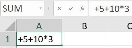
More complex formulas tend to eventually need brackets to achieve the desired result – see the formula in Figure 5.

When Enter is pressed, what result will display in cell A1? What does +5+10*3 equal?

In school, many people learn the calculation sequence that uses the acronym BIMDAS or PIMDAS. This stands for Brackets, Indices, Multiplication, Division, Addition and Subtraction. (Brackets refers to parentheses.)

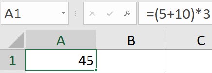
The answer is 35, not 45. This is because the multiplication calculation is done first and returns 30, then 5 is added to return 35. Inserting brackets into the formula calculates 45 correctly, as shown in Figure 6.   

This topic is also discussed in the last month’s Excel Tips column. 

Bracket colour

Always monitor bracket colour when building formulas. A common error is to omit a bracket when creating a formula with multiple functions. 

Excel uses a hierarchy of colours for brackets. The top-level brackets are black. This means that, when typing in brackets, the last bracket should always be black. If there are two black brackets on the end, it means that too many brackets have been added. 

The second bracket colour level is red, and the third level is green. Each function must have both an opening and closing bracket. Make sure they are the same colour. If they are not the same colour, then a bracket is missing.

Don't miss out on more tips, read part two Excel Tips: Formula cheat sheet 2 now.