Loading component...
At a glance
This is part two of a two-part series. Review or catch-up on what you missed in part 1.
Common errors
Two common errors when writing formulas are omitting a comma in a function or omitting quotation marks from around text. All text values that are not cell references, arguments or functions should be enclosed in quotation marks.
For example, =SUM(A1:A10) requires no quotation marks, but =A1 & “Hello” needs quotation marks, because “Hello” is a text value, not a function, argument or cell reference.
Colours on the sheet

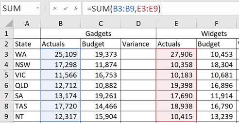
Another use of colours in formulas relates to references. You may have noticed colours on the sheet when creating or editing a formula – see Figure 1.
The coloured ranges serve two purposes – to show where the formula references are on the sheet and to allow those references to be changed.
When editing a formula, point to the border of a coloured range (it will go bold). Then use the mouse to click, hold and drag it to another cell or range. This will update the formula in the Formula Bar.
Another option is to point to the corner of the coloured range and click, hold and drag the arrow icon to change the range reference.
Keyboard vs mouse
There are three ways to enter cell references when creating formulas. All three ways have pros and cons and could be used in a single formula to complete it. The table below explains all three options.
| Method | When to use | Pros | Cons |
|---|---|---|---|
| Use the keyboard to type them | If you know or remember the reference | Quick for keying cell references | Higher risk of making errors, especially with range references |
| Use arrow keys on keyboard | If cells or ranges are close or adjacent to the formula | Quick because the Shift and arrow keys can be used to select a range | Takes longer if cells referenced are far away from the formula |
| Use the mouse to enter them | Every other time | Best technique to access other sheets, as well as cells and ranges not close to the formula | None |
Function Wizard
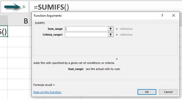
Excel has hundreds of functions. New functions are added regularly to its subscription version. Learn more about a function by using the Function Wizard, which breaks function arguments down into input sections in a dialog and explains each argument.
The Function Wizard also displays the content and results as you build the function – see Figure 2.

Click the fx icon to the left of the Formula Bar after entering a function name to open the dialog.
After completing an argument, a new argument may appear. For instance, SUMIFS requires at least three arguments, but the third argument does not display until the first argument has been entered.
Excel creates the function based on the dialog entries in the Function Wizard – this includes inserting the commas that go between the arguments.
Clicking “Help on this function” at the bottom left of the dialog opens Microsoft’s help page in a browser.
Formula Auditing

Excel has some built-in Formula Auditing tools to help users to understand and debug their formulas. The Formulas tab has a Formulas Auditing section on the right-hand side – see Figure 3.
The Evaluate Formula icon helps to guide users through more complex formulas.
F9 function key

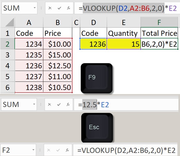
To review a formula in the Formula Bar, select part of the formula and press the F9 function key. This will display the result of that part of the formula. The part of the formula selected must be able to be calculated independently – see Figure 4.
When using this technique, always press the Esc key to reset the formula. Otherwise, the value remains in the formula.
Updated functionality
In the most recent versions of Excel, if the user selects part of a formula in the Formula Bar and that part can be calculated independently, then the result will be displayed above the Formula Bar. It is not necessary to press F9.
Handling errors
Excel formulas can generate many different errors. Excel has two functions that handle errors. The IFNA function handles the #N/A error, and IFERROR handles most errors.

The IFERROR function, shown in Figure 5, prevents the #DIV/0! error that would occur if cell A1 contains zero or is empty.
The downside of using the IFERROR function is that it can mask other issues causing errors by handling all errors the same way.
Dynamic arrays
Excel’s new calculation technique involves working with ranges in the same way users can work with a cell. This causes the formula to spill. A formula can spill down a column, across a row or both, creating a two-dimensional spill range. The formula is only in the top-left cell of the spill range. The other formulas in the range are greyed out and do not exist.
This has implications for the layout of a user’s worksheets, because any entries in the spill range will cause a #SPILL! error.
This topic was covered in detail in a series of three articles:
- Excel tips: how to deal with dynamic arrays
- Excel tips: how to use dynamic arrays' new functions
- Excel tips: how to sort lists using dynamic arrays
New symbols
There are two new formula symbols associated with dynamic arrays.
The @ symbol is placed in front of a function name to force the function to work as it would have before dynamic arrays. Excel may insert this symbol into formulas when the file is first opened with the subscription version.
The # symbol is placed at the end of a cell reference to refer to a spill range. When a formula refers to a spill range, it too will spill to match the spill range.

