Excel Tips: Custom lists and range names

When combined with range names and formatted tables, they can also help automate lists in reports, charts and rosters.

Custom lists can reduce the need to rekey data in Excel. 

For instance, if a user has entered “January” in a cell, dragged the cell and seen the remaining months of the year magically appear in the cells below, they have used a custom list. 

Excel has built-in custom lists for the months and the days of the week. Users can also create their own custom lists.

DIY custom lists

If the list already exists, select it. If it doesn’t exist, then type the entries in separate cells in the sequence that they will be used. 

This example uses a list of states. Follow these steps:

1. With the list selected, press in sequence Alt F T to open the Excel Options window.
2. On the left of the dialog, select the Advanced option.
3. Use the scroll bar on the right side to scroll to the bottom and click the Edit Custom Lists button.
4. Click the Import button – see Figure 1. Click OK and OK again. The list is ready to use.

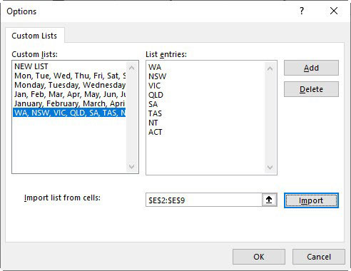
Enter “WA” into a cell and use the Fill Handle to drag the cell to list all the other states. 

The entries can be edited by returning to the Custom Lists dialog. Changing a list does not change any existing lists that have been created. It only updates new lists created. 

Custom lists can be used for departments, branches, products and even staff names.

Custom lists are saved to the computer on which they are created. To use a custom list on another computer, create it again and repeat the process for each computer used.

Range names

There are three ways to capture a custom list in a range name. Once a range has been named, it is no longer necessary to enter a name and drag the list – the range name can populate the whole list. 

Range names are dynamic and can also be used in formulas, as well as across all Excel versions. How they work depends on each user’s Excel version. 

Auto-population is part of dynamic arrays, which is only available with the subscription version of Excel. 

1. Range-based range name

This is the classic way to create a range name. 

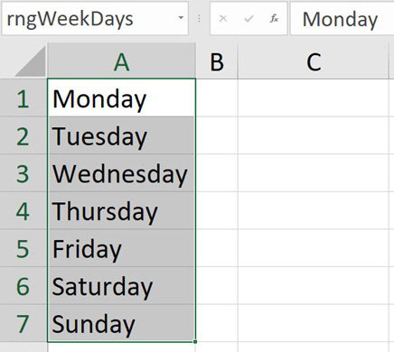
In a sheet, enter the weekday names in a list. Select all the entries in the list and click in the Name Box, to the left of the Formula Bar – see Figure 2. Type rngWeekDays and press Enter.

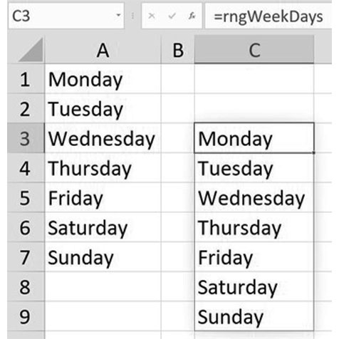
The name rngWeekDays can used throughout the file in a formula to create a list of the weekdays – see Figure 3.

This is a spill range, a dynamic array feature. 

Learn more about the basics of dynamic arrays and spill ranges at this link.

The spill range will spill down to match the original range.

To make the list spill across, use the TRANSPOSE function – see Figure 4.

If the list in the sheet is changed, then that change will flow through to all the formulas that use the rngWeekDays range name.

A problem with this technique is that if an entry is added to the bottom of the list, it will not update the range name. 

Obviously, the days of the week list will not change, but if this technique is used for departments, it might be necessary to add to the list. See the next technique for a dynamic solution.

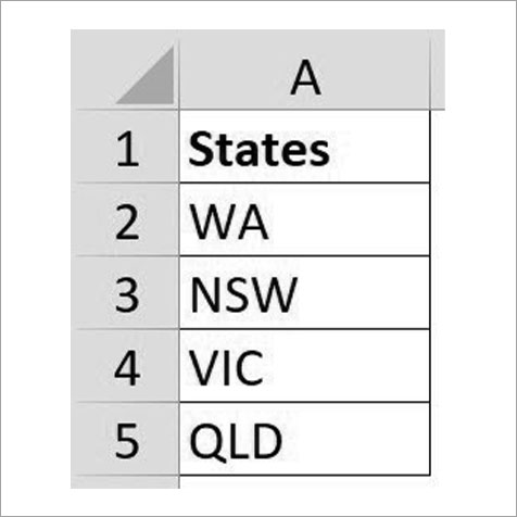
The source for the list in this example is a formatted table. The advantage with this technique is that entries added to the end of the list are automatically included in the range name.

For a list that expands, a heading is recommended – see Figure 5.

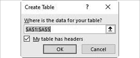
Select a cell in the list and press Ctrl + T. In the dialog box that opens ensure the My table has headers option is ticked and click OK – see Figure 6.

Colour is added to the table, and it is now a formatted table. 

Learn more about formatted tables in detail at this link.

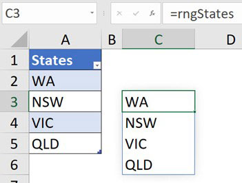
Now select the range A2:A5 (the heading is not included). Click in the Name Box, type rngStates and press Enter. The range is ready to use – see Figure 7.

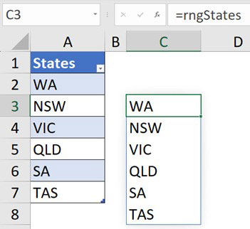
Adding new states to the end of the list updates the range (see Figure 8).

Both techniques work well within the file. However, if a formula with these range names is copied to another file, linking problems between the files may occur. 

3. Self-contained range name  

It is possible to create a list without referring to a range in a sheet. This makes the range name self-contained, allowing it to work in any file without any linking issues.

When creating a custom list inside a range name, it is necessary to use array syntax. Array syntax uses curly brackets (braces) around the entries separated by commas. 

Any text must be enclosed within quotation marks. An example of array syntax is:

{"Mon","Tue","Wed","Thu","Fri","Sat","Sun"}

Typing this structure into a range name is time consuming and prone to errors. The following formula can convert any list of entries into array syntax:

=LET(c,CHAR(34),"{"&c&TEXTJOIN(c&","&c,1,A1:A7)&c&"}")

This formula enables users to copy and paste special values to capture the array syntax without any typing – see Figure 9. It is explained in more detail in the companion video to this article. 

Using copy and paste special values captures the array syntax in a separate cell – see Figure 10.

The subscription version of Excel features a new keyboard shortcut for Paste Special Values – see Figure 11. 

In older versions, use Alt H V V pressed in sequence and not held down.

Copy the array syntax string of characters in the Formula Bar (you may need to press Esc after copying). 

Press Ctrl + Alt + F3 to open the New Name dialog.

Change the name at the top to arrWeekDays.

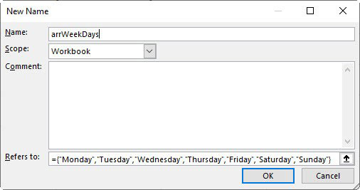
In the Refers to: box, delete everything after the = sign. Paste in the array syntax after the = sign and click OK. The name is ready to use – see Figure 12. 

I have used prefixes to differentiate the range names. 

In a cell, type arrWeekDays – see Figure 13.

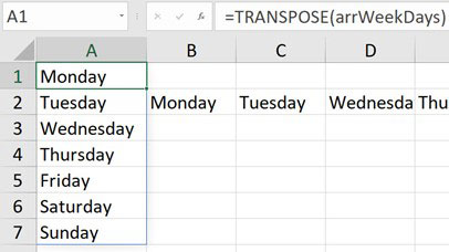
This formula spills across to display all the entries. To display a vertical list, use the TRANSPOSE function – see Figure 14.

If the entries in the range name are changed by editing the array syntax, then all the formulas that use that name will automatically update. To edit a range name, use the Name Manager in the Formulas ribbon tab.

This range name can be used in any file, as it does not rely on a range in a sheet. 

Listing techniques

The following techniques work with all three types of range names. The examples below use the range name arrWeekDays.

The LEFT function can be used to display the abbreviated weekday names – see Figure 15.

The INDEX function extracts from the range name based on the numbers entered in row 1.

Repeating the sequence

Using the range name alone creates a single listing. To repeat the sequence multiple times, a helper cell formula combining the SEQUENCE and MOD functions can be used.

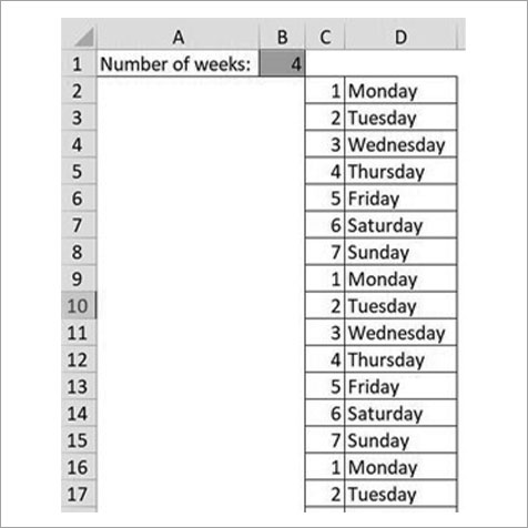
Figure 17 has a vertical listing, which is driven by the number of weeks entered in cell B1.

The formula in cell C2 is =1+MOD(SEQUENCE(B1*7)-1,7)

This creates a vertical sequence of repeating numbers 1 through 7. This formula spills down as far as required, based on the number of weeks entered in cell B1. 

The formula is further explained in the companion video. These are helper cells that make the next formula shorter.

The formula in cell D2 that lists the weekday names is =INDEX(arrWeekDays,C2#)

This formula uses the same INDEX technique as above. It also uses the # reference, which refers to a spill range. This formula will spill down to match the sequence starting in cell C2.

Changing the number in cell B1 changes how many weeks are listed.

Range names are a powerful feature in Excel, and these examples only scratch the surface of their possibilities. 

The companion video and Excel files (blank and completed) will go into more detail to demonstrate these techniques.