Excel tips: using MOD for budgets and forecasts

QUESTION

I use the EOMONTH function to return the month end date. Is there a formula for the quarter end date?

ANSWER 

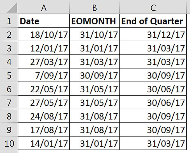
You can hack the EOMONTH function to perform an end-of-quarter calculation. The solution involves a rarely used but versatile function in Excel called MOD. In Figure 1, column A has random dates in 2017. Column B has the EOMONTH function finding the last day of the month for the date in column A.

The formula in B2 is: =EOMONTH(A2,0)

The zero at the end of the EOMONTH function means add zero months to the date in A2 and then determine the month end date.

Before I share the formula in C2, which produces the end-of-quarter date, let’s examine what we need to do. The second part of the EOMONTH function defines how many months to add to the date in A2. The above formula has zero keyed in because it calculates the current month end date. We need a flexible calculation that takes the date in A2 and figures out how many months to add to that date to arrive at the end-of-quarter month for that date. The EOMONTH function will do the rest and calculate the end-of-month date for that end-of-quarter month. 

The solution formula in cell C2 is: 
=EOMONTH(A2,MOD(3-MONTH(A2),3))

This is essentially the same formula as cell B2, except that the zero has been replaced by the MOD function. The MOD function provides the number of months to add to the date in A2 to arrive at the end-of-quarter month. This is a standalone formula that will work with any date. 

The MONTH function in the above formula is straightforward; it returns a number between 1 and 12 representing the calendar month number of the date involved. 

Put simply, any date is either two months, one month or in the same month as the quarter-ending month. The above solution provides the EOMONTH function with a 0, 1 or a 2. 

MOD function

The MOD function is unknown to most Excel users. It performs an unusual calculation that initially may seem useless, yet when used correctly, it offers effective solutions to otherwise complex calculations that involve sequential numbers.  

The MOD function returns the remainder after dividing one number by another. This remainder is surprisingly useful in certain situations. The remainder works counterintuitively for negative numbers. (The formula Excel uses to calculate the MOD function is shown at the end of the article in Figure 4.)

Syntax:
MOD(Number,Divisor)
Number – any value, usually a cell reference or a calculation.
Divisor – the value to divide into the Number.

Examples:
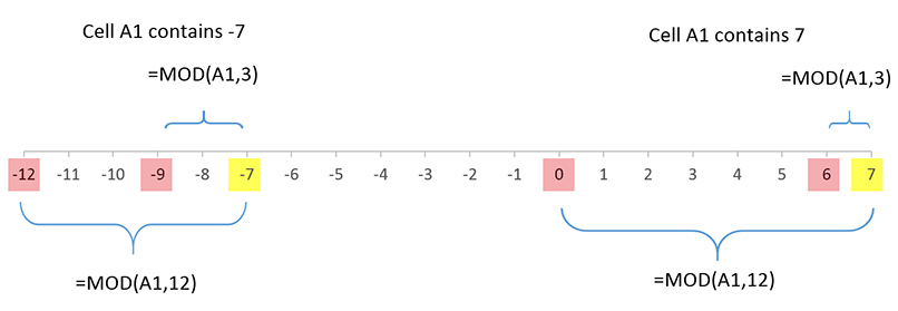
Assume cell A1 contains 7:
=MOD(A1,3) returns 1. Three goes into 7 twice, with a remainder of 1.
=MOD(A1,12) returns 7, as 12 doesn’t go into 7 at all, so 7 is the remainder.

Negative numbers work slightly differently. Assume cell A1 contains -7:

=MOD(A1,3) returns 2. Three goes into -9 three times. The difference between -9 and -7 is 2, so the remainder is 2. The multiple (-9) has to be lower than the Number (-7) to work out the remainder. You don’t use -6 as that value is greater than the Number.

=MOD(A1,12) returns 5, as 12 goes into -12 once. The difference between -12 and -7 is 5. Again, the multiple (-12) has to be lower than the Number. You can’t use zero as that is greater than the Number. 

These last two results are counterintuitive and can take some time to understand, but they will be used as part of our final solution. 

Figure 2 illustrates these examples. The Numbers are highlighted yellow and the multiples used are pink. In that graphic the multiple used must be less than (on the left of) the Number.

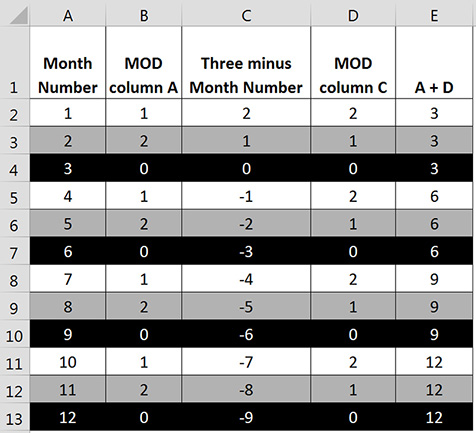
Figure 3 demonstrates how the MOD function works and how it can be manipulated to calculate the correct value to add to the month number to reach the end-of-quarter month. Column A lists the month numbers.  

The formula in cell B2 has been copied down, it is: =MOD(A2,3)

In this formula, the Divisor is 3 because there are three months in a quarter. 

As you can see, there is a pattern in column B. There are only three numbers listed and their sequence repeats. These are the remainders of the month number after dividing by three. This is a standard MOD calculation. This informs us how many months after the previous quarter the current month number is. For example, cell B12 tells us that 11 (Nov) is two months after 9 (Sep). This could be useful for other calculations, but column B doesn’t provide us with the values that we need.

However, we can modify the MOD function to provide the correct values. This technique makes use of how the MOD handles negatives. Column C has a calculation that subtracts the month number in column A from three (the Divisor). 

If you use a MOD calculation on the values in column C, as shown in column D, the MOD function provides exactly the right values we need. 

The formula in cell D2 is: 
=MOD(C2,3)

This calculates how many months we need to add to the month number in column A to arrive at the end-of-quarter month number. Column E shows the quarter-ending numbers by adding the number in column A to the MOD result from column D.

Back to our solution in cell C2 in Figure 1: 
=EOMONTH(A2,MOD(3-MONTH(A2),3))

This uses an EOMONTH function with the date from column A. The MOD function subtracts the month number of the date in column A from 3 and finds the remainder after dividing by 3. This is the number of months we need to add to the date in column A to arrive at the end-of-quarter month. The MOD in this formula combines columns A, C and D from Figure 3 into a single formula.  

Sequences

If you are dealing with numbers that have regular sequences, the MOD function can help identify patterns that may not be obvious. Subtracting the Number from the Divisor, as we have done, can provide a simple solution that would otherwise require a more complex formula.

The MOD function can be used in budgets and financial models to handle periodic payments: bi-monthly, quarterly or semi-annual. Note in Figure 2 that in column B each time a multiple is reached the MOD returns 0. This can be a simple test for an IF function to identify months that are bi-monthly, quarterly or semi-annual.

Figure 4 shows the formula used to calculate the MOD result. The INT reference in the formula rounds a number down to the nearest whole number. So (n/d) is rounded down to the lowest whole number. For negative numbers, this means rounding away from zero, so both -0.33 and -0.66 would be rounded to -1. 

The companion video and an Excel file may assist your understanding.

Neale Blackwood CPA runs A4 Accounting, providing Excel training, webinars and consulting services to organisations around Australia. Questions can be sent to [email protected]