Excel tips: how to use SUMIFS and EOMONTH for sales trends

QUESTION

I have a table containing daily sales for a number of years. I want to create a Moving Annual Total report by month and year. What formula would I use?

ANSWER 

The SUMIFS function in combination with the EOMONTH function provides enough calculation flexibility to create your report.

Moving annual total (MAT) reports are a common way to remove seasonal variations. Quarterly figures tend to be affected by seasonal factors. When you are reviewing MAT figures you are always looking at 12 months’ data, which makes the figures more comparable. 

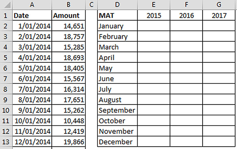
Figure 1 shows the sales data in columns A and B. The report structure starts in column D. We will create a formula in cell E2 that calculates the annual sales till the end of January 2015. This formula will be copied across and down to complete the report. 

The SUMIFS function performs multi-criteria summing calculations. In our case we need to provide a starting date and an ending date to calculate the 12 months’ sales. You might think a PivotTable could be used to create the layout we’re after. Our report splits the dates between the month (column D) and the year (row 1). We can’t create a PivotTable in that structure with the existing data.

The formula for cell E2 is:
=SUMIFS($B:$B,$A:$A,”<=”&EOMONTH($D2&E$1,0),
$A:$A,”>=”&EOMONTH($D2&E$1-1,0)+1)

I have used references to whole columns in this formula to shorten the formula. The $ signs in the formula fix whichever reference they are in front of. Because we need to copy this formula down and across, the position of the $ sign is important.

For example, cell D2 contains January. To enable us to refer to that cell as we copy it across we need to ensure column D doesn’t change, so we put the $ sign in front of the D ($D2). We want the reference to row 2 to change as we copy it down so there isn’t a $ sign in front of the 2.

Breaking down the SUMIFS function

Let’s break the SUMIFS function down into its five arguments and look at how each works.
=SUMIFS($B:$B

The first argument in the SUMIFS function is the range to sum. In our case it’s column B.
$A:$A

The second argument in the SUMIFS function is the range that contains the first criteria. In our case that is column A. In fact, both our criteria ranges use column A, because the criteria is date driven.
“<=”&EOMONTH($D2&E$1,0)

The third argument in the SUMIFS function is the first criteria that we are looking for in column A. 

When using the “less than or equal to” symbols <= in the SUMIFS function, you must enclose them in quotation marks and join them to the date, or value, that you are comparing. I have used the & symbol to join text together.

We need to create a date for the end of January 2015. Luckily, Excel includes a function that extracts the end of month date from a given date.

The EOMONTH function has two parts to it: the first is the date that you want to work with, the second is how many months you want to add to that date. In our case we don’t want to add any months to the date, so we have a zero at the end of the EOMONTH function.

I have used a date hack to create the date that we want to use:
$D2&E$1

This part of the formula creates a string, January2015. When you use a string where Excel is expecting a date, Excel will try to convert that string into a date. In our case, the structure that I have used is one that Excel recognises. Excel defaults to the first of the month if a date doesn’t include a specific day.

The EOMONTH function returns the last calendar day of the month for the month involved. In our case, EOMONTH($D2&E$1,0) will return 31 January 2015.
$A:$A

The fourth argument is the second criteria for our SUMIFS function. It uses the date column again.
“>=”&EOMONTH($D2&E$1-1,0)+1

The fifth and last argument is the starting date for the 12 months’ sales. In our case, that would be 1 February 2014. We can also use the EOMONTH function to create that date.
$D2&E$1-1

This part of the formula creates a string for January2014 (the year before), because we subtracted 1 from E1.
EOMONTH($D2&E$1-1,0)+1

The EOMONTH provides the end of month for January 2014 (31 January 2014) and we added 1 to that date, which will become 1 February 2014.

The SUMIFS function will add up all the values in column B when the date in column A is less than or equal to the 31 January 2015 and greater than or equal to 1 February 2014.

These dates will vary as the formula is copied down and across to populate the rest of the report.

Once you have summarised the data into MAT figures, you could use charts to assist in identifying trends and relationships. 

Another date hack

You can convert a text month, for example, July, into a month number (7) using the following date hack. Assuming A1 contains the word July, the following formula will return 7:
=MONTH(1&A1)

By joining 1 to the front of a month name, you are creating another date structure that Excel recognises. If you type 1July in a cell, Excel will convert it into 1 July for the current year.

The MONTH function returns a number from 1 to 12, representing the calendar month number. This will work even if A1 contains Jul.

If you require the financial year month (July = 1 and June = 12), you could use: 
=MONTH(1&A1)+IF(MONTH(1&A1)>6,-6,6). 

The companion video and Excel file may assist your understanding.

Neale Blackwood CPA runs A4 Accounting, providing Excel training, webinars and consulting services to organisations around Australia. Questions can be sent to [email protected]