A smarter way to calculate grand totals in Excel

Most people use the SUM function when subtotalling, however the grand total calculation can be an issue when rows are inserted within the range. Excel’s SUBTOTAL function solves this.

Syntax:

SUBTOTAL(Function _Num, Ref1, [Ref2])

Function _Num – a number that specifies the function to use in the calculation. In most cases, 9 or 109 are used as they represent the SUM function in Excel.  

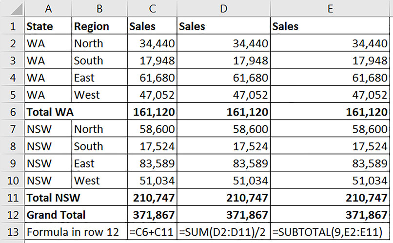
Ref1, Ref2 – range(s) to perform the calculation on. Any SUBTOTAL functions within these ranges will be ignored. Since the SUBTOTAL function ignores all other SUBTOTAL functions within its range, it means the grand total formula is much simpler than if you use a SUM function. See Figure 1.

The values in columns C, D and E are the same. Columns C and D have SUM functions in rows 6 and 11. Column E uses the SUBTOTAL function in rows 6, 11 and 12. Row 13 lists the formulas in row 12. 

Issues with the grand total row

Column C – if a new section is added to the data you must remember to add it to the grand total calculation at the bottom.
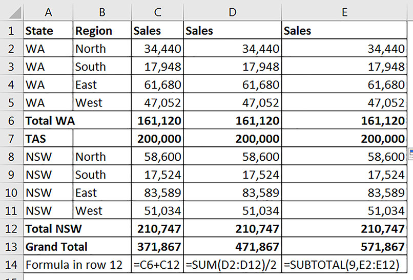
Column D – the SUM function adds up the whole range and divides by two. This assumes that there are value rows followed by a subtotal row for each section. If a single row is added with a value and no subtotal, then the grand total will be wrong.

In Figure 2 I have inserted a row for Tasmania. It doesn’t have regions, so it has a single entry.

The table on the right of Figure 3 has been filtered by WA and NSW. 

The formula in cell B11 is =SUBTOTAL(9,B2:B9). 

This calculation automatically adjusts to sum just the visible cells as the filters change. Had you used =SUM(B2:B9) it would display 2447 no matter what filter is applied.

Filter by colour

Many people are unaware that you can filter by colour in Excel. You can either manually format the cells or you can use conditional formatting. The formats can then be used to filter the list and have SUBTOTAL add up the filtered values. 

Visible cells

The SUBTOTAL function has the ability to add up only the visible cells. We saw that SUBTOTAL ignored rows hidden by a filter. It can also ignore all hidden rows or columns and just add up visible cells. To add up visible cells only, use 109 instead of 9. Figure 4 shows an example.

The formula in cell C7 is =SUBTOTAL(109,C2:C5) and this has been copied across to column D.

On the right of Figure 4 I have hidden rows 3 and 4. The SUBTOTAL automatically adjusts.

This is useful if you have a spreadsheet with hidden rows or columns and you want to check if there are any values in those hidden cells. By comparing a SUM function on a range with SUBTOTAL using 109 you can see if there are values in the hidden ranges.

Automated subtotals

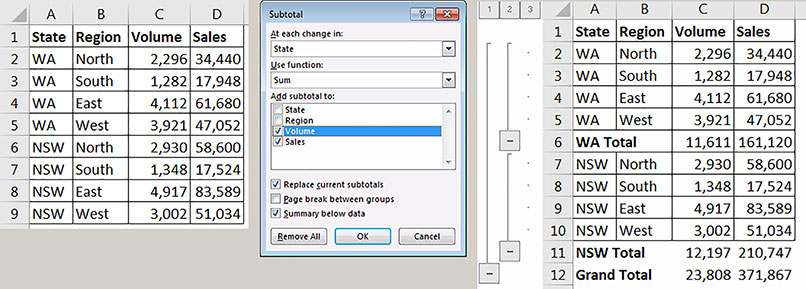
If you have a list that you want to subtotal, Excel can do all of the work for you. This technique requires that you sort your list by the field that you want to subtotal by. With a sorted list you can automatically insert subtotals using the Subtotal option. This is on the right-hand side of the Data ribbon tab. The keyboard shortcut to open the Subtotal dialog is Alt A B, pressed in sequence, not held down. See Figure 5.

Rows 6, 11 and 12 all have SUBTOTAL functions added. You may need to tick more value columns in the middle of the Subtotal dialog, these are columns that are added up. Otherwise the other options are usually correct. If you want to remove the subtotals, go into the dialog and click Remove All. Excel also adds the grouping icons on the left. 

Note: The cell border format is not copied down.

Common questions

I regularly hear two questions regarding automated subtotals:

1. How do you copy and paste just the subtotal rows? First, use the grouping buttons to show just the subtotals. Select the range involved, hold down the Alt key and press the semi-colon. This shortcut selects just the visible cells. You can then copy and paste as normal. After you copy, the selected range may look unusual in that the dotted lines display within the range.

Note: The pasted range will only include values, no formulas are pasted.

2. When using automated subtotals how do I make the subtotal values bold like the labels? Use the grouping icons to display just the subtotals then select the values range and press then Alt + ; to select visible cells only. Then use Ctrl + B to bold the selection.

A limitation of automated subtotals

You can’t use automated subtotals in a formatted table. A formatted table is one created using the Format As Table icon on the Home ribbon. While you can’t use subtotals within a formatted table, you can add totals to the bottom of a formatted table. Select a cell in a formatted table; in the Design ribbon tab that displays, there is an option to add totals to the formatted table.

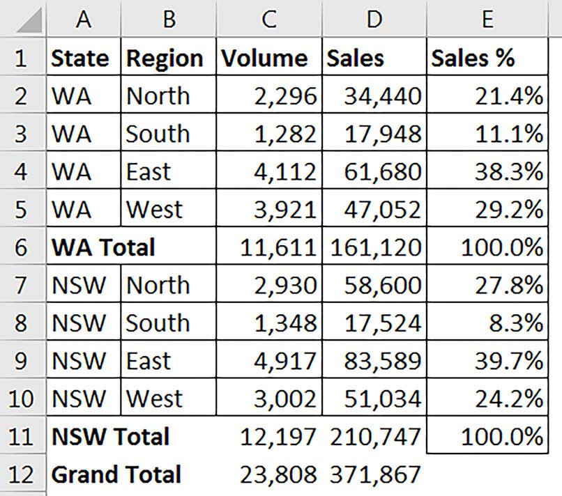
In Figure 6 I have added sales percentages to the table from Figure 5. The formula in cell E2 calculates a percentage within each subtotalled section and it can be copied down the whole range. I will explain how the formula works in the companion video above.

The formula in cell E2 is 
=D2/VLOOKUP ("*Total",$A2:$D$12,4,0) 

The companion video and Excel file will go into more detail to demonstrate these techniques.

Neale Blackwood CPA runs A4 Accounting, providing Excel training, webinars and consulting services to organisations around Australia. Questions can be sent to [email protected]