Excel tips: how to use the SUMIFS function

The SUMIFS function is used to summarise large data sets in table structures. There are other functions that handle multi-criteria calculations. They have a similar structure to SUMIFS. They are AVERAGEIFS and, in more recent versions, MAXIFS and MINIFS.

In many cases, the report you create with a SUMIFS can be created using a PivotTable. The problem with PivotTables is that their structure is inflexible and the simple act of inserting a column is not allowed. PivotTables also require a Refresh if the data changes.

Formula-based reports that use SUMIFS can be laid out exactly as you require, and they will automatically calculate.

Syntax

SUMIFS (sum_range, criteria_range1, criteria1, criteria_range2, criteria2 …)

sum range – the range that contains the values to add up. Typically this range is a fixed reference, that is, it uses the $ sign to ensure the rows and columns do not change. When all the criteria are met in all the criteria ranges, the value in this range is added up.

criteria range# – the range(s) that contains the criteria entries to be compared with the corresponding criteria. Typically these ranges are also fixed references.

criteria# – typically a cell reference that contains the entry to be searched for in the corresponding criteria range. This cell reference is usually a fixed or a mixed cell reference.

All the ranges must line up, and start and end on the same rows for vertical data. The start and end columns must line up for horizontal data. You can also refer to whole columns or whole rows.

Examples

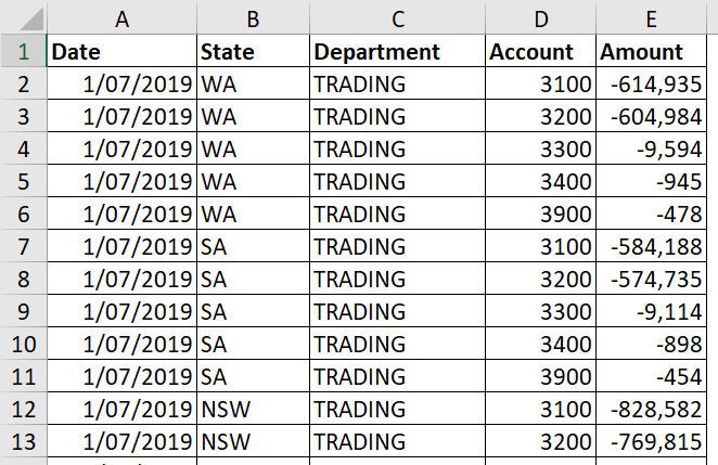
We will use the dataset in Figure 01 for the examples. The data goes down to row 735. Figures 02 and 03 are on the same sheet as this data.

Example formulas are displayed in Figure 02. Column K uses the FORMULATEXT function to display the formulas in Column J. 

Formula explanations

Row 2 shows a single-criteria SUMIFS. Note both ranges refer to the same row numbers. This is important. If the rows do not align, an error is returned. When WA is found in Column B, the corresponding value from Column E is summed.

Row 3 has a two-criteria SUMIFS. An extra criteria has been added for the date. When the date in Column A is 1/7/2019 and Column B has WA, then the value in Column E is summed.

To add an extra criteria, you add an extra criteria range and criteria to the end of the SUMIFS function. Row 4 has a three-criteria SUMIFS, with the added criteria for the TRADING department in Column C of the data.

Whole columns

You can refer to whole columns in the formula. This has the advantage of shortening the formula and removing the possibility of missing data if extra data is added to the bottom of a range. The downside is that it may affect calculation speed.

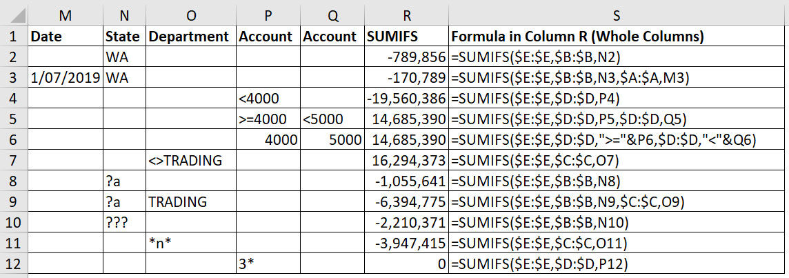
In Figure 03, I have rewritten the top two formulas from Figure 02 in a separate table, using whole column references. The other examples in this table also use whole column references to shorten the formulas. You can only use whole column references when there is no other data under the existing table.

Using comparison operators

Most criteria require that the criteria range equals a value. In row 3 of Figure 02 and Figure 03, we sum Column E when the Date and State equal their respective criteria.

In some cases, especially when using dates or account numbers, you may need to use the greater-than and less-than symbols to extract the correct data. When using these symbols, you can incorporate them into the criteria cell or enclose them in quotation marks within the formula.

Rows 4 and 5 in Figure 03 demonstrate how to use the symbols within the criteria cell. Row 4 sums Column E when the account number in Column D is less than 4000. 

Row 5 sums Column E when the account number in Column D is greater than or equal to 4000 and less than 5000.

Row 6 performs the same calculation as row 5, but the symbols have been included in the SUMIFS function. When using the symbols like this, they must be enclosed within quotation marks and you use the & symbol to combine the symbols with the entry in the cell. The & symbol joins text together. Note the two criteria ranges are the same because there are two criteria being applied to the same column.

Row 7 has an example of not equal to. This is represented by the less-than symbol followed by the greater-than symbol. This formula adds all the values in Column E where the Department isn’t TRADING.

Wildcards

Excel has two wildcard characters. They are ? and *. These represent unknown characters and can be used with the SUMIFS function to provide more flexibility. The ? represents one unknown character. The * represents any number of characters and even no characters.

Row 8 adds up the states that have two characters and the second character is an a. Note this is not case-sensitive. This will include WA and SA. TAS would not be included as it is a three-character code.

Row 10 adds up all three character state codes, and in the data this includes NSW and VIC. Row 11 uses the * wildcard character, which represents any number of characters including no characters. This will add up any department code that contains n in any position. If there was a department code with just the letter N, it would also be included. You need to be careful using the ? and * with numeric codes. Row 12 seems to be adding up all the account numbers starting with 3. It returns zero because the wildcards don’t work with numeric codes. They will work with alphanumeric codes.

Limitations

SUMIFS has two limitations.

1. It doesn’t work on closed workbooks. This also applies to the other conditional functions mentioned at the start of the article. If you are using external file ranges, the files must be open for the SUMIFS to return a result. The SUMPRODUCT function can perform similar calculations, and it works on closed workbooks.
2. It doesn’t handle leading zeros in codes correctly. If you had codes 00123, 0123 and 123 in a column, they would all be included in a 123 condition. I will demonstrate this limitation in the companion video. The SUMPRODUCT function handles leading zeros correctly.

The companion video and Excel file will go into more detail to demonstrate these techniques.

Neale Blackwood CPA runs A4 Accounting, providing Excel training, webinars and consulting services to organisations around Australia. Questions can be sent to [email protected]