Loading component...
At a glance
Recently, I was solving a date problem in a table. I needed a formula to conditionally find the earliest date that matched two other criteria from a table. The solution would depend on which Excel version I am using.
Over the past 10 years, Excel has changed dramatically. Now more than ever, your software version determines what you can do and how easy the solution is.
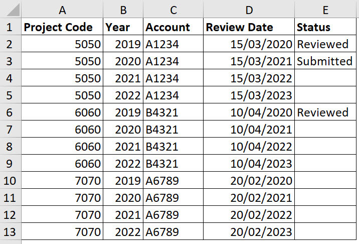
The table I am working with is shown in Figure 01.

I need to know the next Review Date for each project. That means I need the earliest date in column D, where there is a blank cell in column E.
My report is shown in Figure 02. The columns contain four different solutions. Row 1 has the versions they work in. Row 2 describes the solution.

All the formulas from row 4 in Figure 02 are shown in Figure 03.

The row 4 formulas have all been copied down. You will need to refer back to Figure 03 as I explain these formulas. The formulas are reasonably complex, and I provide more detail in the companion video to this article.
The formula from cell K9 has not been shown yet and will be handled last.
To identify or return a blank cell, you use two quotation marks together like this: "".
All versions - array - column H
Array formulas are more complex than most formulas. Array formulas can work with ranges in the same way that standard formulas work with single cells. You must use a special keyboard combination to enter arrays.
Hold down the Ctrl and Shift keys and then press the Enter key. That places the braces (curly brackets) around the formula. You can see them in the first formula listed in Figure 03.
This array formula first calculates the first IF function. This compares each cell in the range A2:A13 with the project code in cell G4. If a cell matches the project code, it goes to the next IF function and looks in the corresponding row in the range E2:13 for a blank cell.
If it finds a blank cell, then the corresponding row from D2:D13 is returned. If either of the tests are FALSE, a blank cell is returned.
Together, the two IF functions provide a range of dates and blank cells for the MIN function (which returns the minimum value) to review. The MIN function ignores blank cells.
The remaining dates are compared to determine the earliest (minimum) date. This type of calculation with normal formulas would take multiple cells to perform. An array formula can do all the calculations in a single cell.
Excel 2010 and later - aggregate - column I
The AGGREGATE function has the unusual ability to ignore error cells. This ability enables us to build a single formula that works like an array formula but is not an array.
The AGGREGATE function is like the SUBTOTAL function. You specify which calculation to perform. The “15” at the start defines the SMALL function. The SMALL function is a flexible version of the MIN function.
The MIN function returns the minimum value in a range. The SMALL function can find the lowest, or the second lowest, by specifying a position number: 1 finds the lowest, 2 the second lowest.
The second argument of AGGREGATE has 6, and this instructs it to ignore errors.
In Excel, dates are numbers. Each date has an underlying sequential number. In the AGGREGATE function, we are dividing the date range by the result of a conditional calculation. That calculation looks at two separate conditions. Here’s how that calculation works.
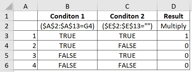
Each cell in the range can return TRUE or FALSE. When we multiply the two conditions together, they convert TRUE into 1 and FALSE into 0. The result from A2 will be multiplied by result from E2 and so on down the ranges.
With two conditions, there are four possibilities and two possible results, as seen in Figure 04.

When you multiply anything by zero (FALSE), it returns zero, as you can see in Figure 04. The only time 1 is returned is when both conditions are TRUE.
We divided the dates by these condition results. Any condition that didn’t match will be zero. Dividing by zero returns an error.
We instructed the AGGREGATE function to ignore errors. When both conditions match, the date will be divided by 1, which leaves it unchanged. The remaining dates will match both criteria. They are analysed by the SMALL function to determine the lowest date.
The 1 at the end of the AGGREGATE function instructs the SMALL function to return the lowest (earliest) value from the dates.
The IFERROR function has been added to handle the error generated when no conditions are met.
This occurs when there is no blank cell for a particular project code.
Excel 2019 and later - MINIFS - preferred solution - column J
Just as the SUMIFS function allows conditional summing, the MINIFS function allows a conditional minimum calculation.
The first range, D2:D13, is the range in which to find the minimum.
Then you pair up a condition range, A2:A13, with a condition G4. You add conditions by adding another condition range, E2:E13, and another condition, "". These are all separated by commas.
Since this function has been created to handle our requirement, it is my recommended solution. Unfortunately, it is only available in Excel 2019 and the subscription version. Note that there is a MAXIFS function as well.
Subscription version only - dynamic arrays - column K
The subscription version of Excel is available through Microsoft 365 (formerly Office 365). This version receives regular updates. In 2020, it received the dynamic arrays update, which I covered in three separate articles in May, June and July 2020.
Dynamic arrays change the way formulas are calculated. In terms of array formulas, you no longer need to use Ctrl + Shift + Enter to enter them. The formulas in cells H4 and K4 are identical except for the braces on either end.
The calculation in the subscription version works the same as the array formula I described earlier. I do not recommend using this dynamic array solution, because we have the specialist MINIFS function available in the subscription version.
This formula shows that Excel’s new calculation engine can handle a single cell formula that works with conditions based on ranges, not just single cells. I included it, so you can see how we can adapt it to handle a more difficult requirement.

Let’s say that, instead of finding the first date based on a project code, we want to find the first date based n the first letter of the Account code in column C. Perhaps different prefixes relate to different account categories. Figure 05 has the report. The formula in K9 is included in Figure 03. The MINIFS function cannot handle this type of condition.
Dynamic arrays allow you to manipulate ranges with other functions. The LEFT function extracts characters from the left of a cell. We can use it to extract the first character from the Account column range.
We can replace the project code condition with a condition that extracts the first character from each cell in the range C2:C13. This is then compared to the letter in cell J9 to return TRUE or FALSE for each cell in the range.
Excel has progressed over the years. We moved from array formulas, which are complex and require a special keyboard entry, to a function that works like an array and then to a dedicated function built to handle conditional minimum calculations.
Finally, Excel has formulas that can handle flexible conditions on ranges using dynamic arrays.
Remember to watch the companion video to this article, which will go into even more detail about how these formulas work.
The companion video and Excel file will go into more detail to demonstrate these techniques.
Neale Blackwood CPA runs A4 Accounting, providing Excel training, webinars and consulting services. Questions can be sent to [email protected]

