Bonus Excel tips: 3D SUMIFS, range names and the TODAY function

1. Create 3D SUMIFS for multiple worksheets

Back in 2005, I shared a complicated formula to perform a simulated 3D SUMIF – to sum a column of values based on the codes in another column through multiple sheets.

This was back before the SUMIFS function existed. The solution is a bit of a hack because there is no easy way to do a 3D SUMIF in Excel. SUMIF is a conditional SUM.

I no longer use SUMIF. I always use and teach SUMIFS. SUMIF only allows one condition, while SUMIFS allows up to 64 conditions. SUMIF and SUMIFS have a slightly different syntax. 

For these reasons, I will use SUMIFS in this tip.

This tip also uses the INDIRECT function. 

Many people don’t know about the INDIRECT function. 

Others avoid it because it is a volatile function. This means INDIRECT functions recalculate each time Excel calculates. 

Most functions only recalculate if a value in their range changes. Volatile functions can slow Excel down, but this is less of an issue now than it used to be.

INDIRECT also stops you being able to audit the formula. Excel has a built-in auditing feature that allows you to track where values are coming from. When you use INDIRECT, you can’t follow the links.

For these reasons, INDIRECT tends to be a last resort. If you can’t perform a calculation with Excel’s built-in formulas, INDIRECT will often provide a solution.

Note: INDIRECT is probably the worst named function in Excel. Its name has no relationship to what it does. 

The INDIRECT function converts the text between its brackets into a cell or range reference. 

As an example, =INDIRECT("A10") refers to cell A10. This isn’t that useful, but if cell A1 contains the text A10 then =INDIRECT(A1) refers to cell A10 and changing cell A1 to A100 would update the INDIRECT to link to A100. 

This is more useful as you can update a cell text entry to change a link in another formula without having to edit the other formula.

Let’s have a look at a much more complex problem. You might need to read this several times or watch the companion video a few times to understand this, as it involves a complex technique. 

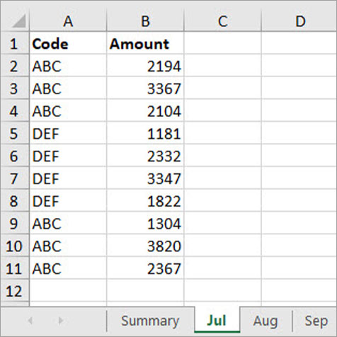
There are three sheets named Jul, Aug and Sep – see Figure 1.

All three sheets have the same layout with codes in column A and values in column B.

In a separate Summary sheet (Figure 2), we want to add up all the values in column B of all the month sheets that match the code in column A. 

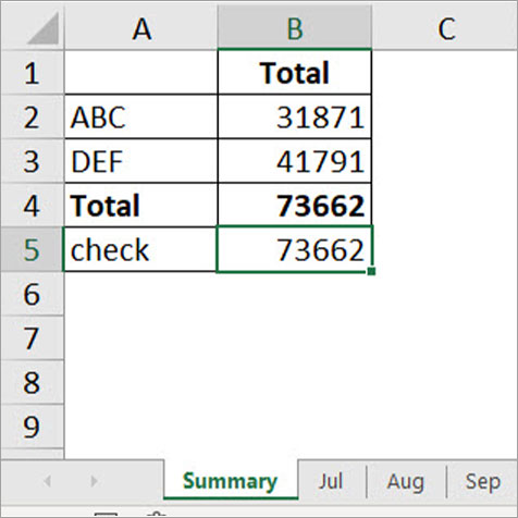
Normally, this would require three separate SUMIFS functions added together. However, we can use a single INDIRECT function to create a formula that works like a 3D SUMIFS. 

In the Summary sheet, the formula for cell B2 is

=SUM(SUMIFS(INDIRECT({"jul","aug","sep"}&"!B:B"),INDIRECT({"jul","aug","sep"}&"!A:A"),A2))

Note: I have used full column references to shorten the formula. Let’s unpack the various parts of this formula.

{"jul","aug","sep"}&"!B:B"

This part of the formula creates three separate text strings.

“jul!B:B”

“aug!B:B”

“sep!B:B”

The use of the curly brackets is called array syntax. This array syntax instructs Excel to create three separate ranges. All three have !B:B on the end but start with the three entries between the curly brackets.

INDIRECT({"jul","aug","sep"}&"!B:B")

The INDIRECT then converts these three text strings into three separate range references referring to column B in the three separate sheets.

The INDIRECT on the end creates these range references. 

jul!A:A

aug!:A:A

sep!A:A

SUMIFS(INDIRECT({"jul","aug","sep"}&"!B:B"),INDIRECT({"jul","aug","sep"}&"!A:A"),A2)

This part of the formula creates three separate SUMIFS functions

SUMIFS(jul!B:B,,jul!A:A,A2)

SUMIFS(aug!B:B,aug!A:A,A2)

SUMIFA(sep!B:B,sep!A:A,A2)

The SUM at the start of the formula adds the result of the three SUMIFS functions together to provide the solution, which can be copied to cell B3 in the Summary sheet.

True 3D calculation

The Summary sheet has a 3D SUM function. The check formula for cell B5 is

=SUM(Jul:Sep!B:B)

This is a true 3D formula. It sums column B in all the sheets from Jul to Sep inclusive. If you inserted more sheets between Jul and Sep they would be included in the calculation. This is the only type of calculation in Excel where the position/sequence of the sheet makes a difference to the result.

All Excel’s basic functions, like COUNT, AVERAGE, MIN and MAX, can perform these 3D calculations. More complex functions like SUMIF and SUMIFS cannot. 

Update

Before the subscription version of Excel, you had to type in the array syntax to formulas. 

Now we can use a formula to insert array syntax. This makes it more flexible. 

In Figure 3 there is a slightly different structure in the Summary New sheet. 

The formula in cell B2 is

=SUM(SUMIFS(INDIRECT(SORT($E$1:$G$1)&"!B:B"),INDIRECT(SORT($E$1:$G$1)&"!A:A"),A2))

The SORT function provides the array syntax for the three sheet names. This makes the solution much more flexible.

You may have noticed in Figure 3 that I have added an Oct sheet tab. 

In Figure 4, I have amended the structure by inserting a column and updating the sheet names to include Oct. 

The formula for cell B2 is now

=SUM(SUMIFS(INDIRECT(SORT($E$1:$H$1)&"!B:B"),INDIRECT(SORT($E$1:$H$1)&"!A:A"),A2))

This adds up the four sheets Jul, Aug, Sep and Oct.

In Figure 4, I also updated the check cell B5.

=SUM(Jul:Oct!B:B)

2. The quick way to create range names

Once you start using range names in Excel, you will find there are many uses for them. 

You can create them using the Name Box and the Define Name dialog box, but Excel also has a built-in feature to speed up the range name creation process.

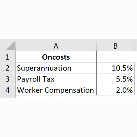
In Figure 5, we have three oncost percentages. 

We want to name each cell in column B with the label shown in column A, so, for instance, cell B2 will be named Superannuation. 

Note that the other labels include spaces, but spaces are not permitted in range names, so Excel will insert the underscore character instead of the space character.

Select the range A2:B4 and click the Formulas ribbon tab. In the middle of the tab in the Defined Names section, click the Create from Selection icon. A dialog will display. 

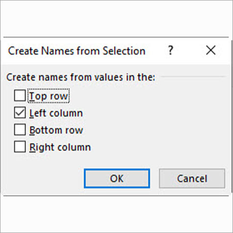
Make sure only the Left column option box is ticked, because the names we want to use are in the left column of the range we have selected – see Figure 6.  

Click OK and Excel will create three range names in one step.

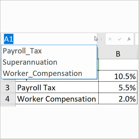
The Name Box on the left of the Formula Bar has a drop down. If you click it, you can see the three new names listed – see Figure 7.

The range names are listed in alphabetical order. Note the use of the underscore character.

Abbreviations

You may want to use abbreviated names rather than the full name, e.g. Super, PRT, WComp. In that case, insert a column between the label and the value and enter the abbreviated names. 

Use that column to create the range names. When I do this, I change the font colour, use italics and label the column as Range Names – see Figure 8.

Keyboard shortcut

To open the Create from Selection dialog from Figure 6, we can use the keyboard shortcut Ctrl + Shift + F3. 

Range name rules

Range names in Excel cannot:

• start with a number
• contain spaces
• use symbols, except full stops or underscores
• be a cell reference, e.g. Q1 and QTR1 are both cell references. Use Q_1 or QTR_1

It is a good idea to:

• Start the range name with an uppercase letter, such as Expenses
• Use an uppercase letter for the first letter of each word, such as TaxRate

The reason I recommend using at least one uppercase character is that if you type a name in lowercase and press Enter, Excel will change the case if it recognises the range name. 

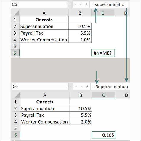
This is like entering a function name in lowercase. If you make a typing error, the name will remain in lowercase and the #NAME? error will display – see Figure 9.

In cell C6, in the top section the “n” has been omitted and the cell displays the #NAME? error. Note the name is still all in lowercase. 

Adding the “n” to the end fixes the spelling, removes the error, and capitalises the first letter. This is useful if you use multiple range names in a formula and it is displaying an error. 

When you always use an uppercase character in all your names, if a name is still in all lowercase then it is the problem.

3. Use the NOW and TODAY functions to display the current date

The =NOW() function is used to update the current date in a spreadsheet. In Excel, dates are numbers. Day 1 was 1 January 1900. Each day since has a sequential number. Remembrance Day in 2022 has the number 44876 – see Figure 10.

Fractions show up using the NOW function because time is treated as a fraction of the day. 6 am is 0.25, noon is 0.5 and 6 pm is 0.75. You can see the fraction for 11 am in cell D2 in Figure 10.

To show today’s date without a fraction, you can use the TODAY() function, as in cell C3 of Figure 10.

To remove a fraction from a number, you can also use the TRUNC function. TRUNC is short for truncate. 

The TRUNC function cuts off the fraction. It doesn’t round the number like the ROUND function. The TRUNC function removes the fraction completely leaving the whole number unchanged – see Figure 11.

Both NOW and TODAY are volatile functions like the INDIRECT function.

The companion video and Excel files (blank and complete) will go into more detail to demonstrate these techniques.