Loading component...
At a glance
I answered three questions between February and April 2005.
1. How can I put the full path name of my file in the footer without typing it?
Answer: This is a lot easier these days than it was back then. There are a couple of easy ways to access the Header and Footer options now.

On the Insert ribbon tab, there is a Header & Footer option on the far right-hand side. See Figure 1.
Clicking this icon changes the view to Page Layout, which makes Excel look like a Word document, as per Figure 2.
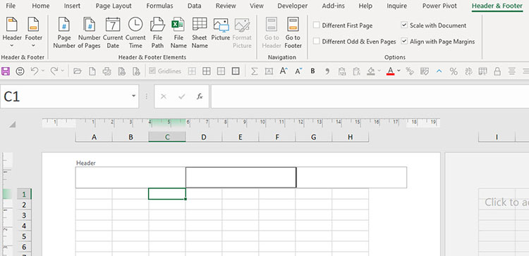
This view allows you to see the sheet as it would be printed, including page margins. You can click in the header or the footer section to access the header and footer options.
The header and footer have three sections, left, middle and right. You can use the icons in the ribbon at the top to insert the different information required.
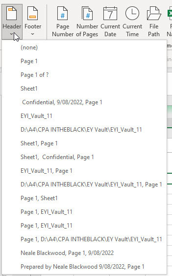
The header and footer icons on the far left have some standard header and footer settings you can select from. See Figure 3 for the standard header options.
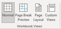
There are a couple of other ways to get to the Page Layout view. In the View tab, there are three view icons – Normal, Page Break Preview and Page Layout - see Figure 4.
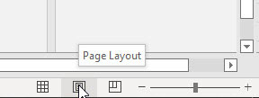
You can also access the Page Layout view using the middle icon on the bottom right of the screen near the zoom controls – see Figure 5.
To return to the Normal view, click the first icon.
2. I have a range of cells that contain formulae and values. I need to multiply all the cells in the range by a factor. The factor could change. Is there an easy solution?
Answer: The solution provided then is still relevant today. It involved a range name.
Let’s use the structure in Figure 6 as an example.
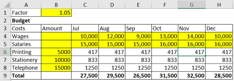
The yellow cells are input cells and the other value cells contain formulas. We want to apply a factor to the range C4:H8. The factor value is in cell B1.
We will name cell B1. Select cell B1 and click in the Name Box. The Name Box is on the left of the Formula Bar. It usually displays the cell reference. Overwrite the cell reference and type Factor into the Name Box and press Enter – see Figure 7. Pressing Enter is important. If you just click outside the Name Box the name will not be defined.
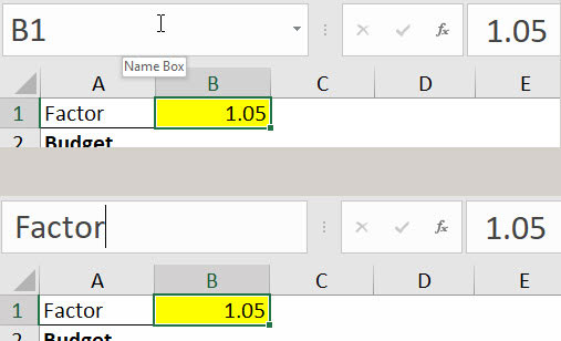
Now the cell has been named we can use the name in a formula.
To apply the factor to all the cells, follow these steps.
- In cell D1 type =Factor and press Enter.
- Select cell D1 and copy it.
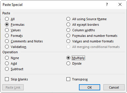
- Select the range C4:H8. Press Ctrl + Alt + V this opens the Paste Special dialog.
- Select Formulas in the top section and Multiply in the middle section and click OK. See Figure 8.
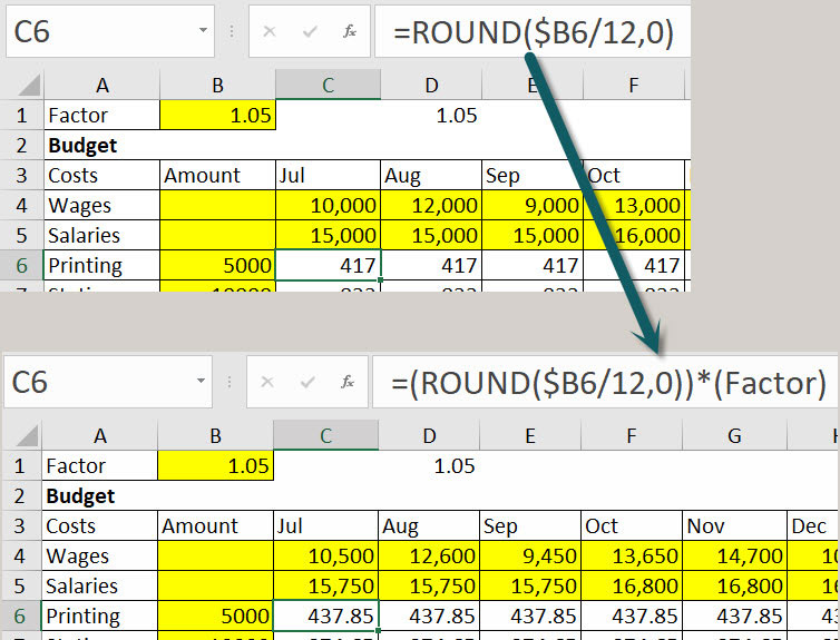
The input cells and the formula cells within the range will all be adjusted so that they are multiplied by the Factor. See Figure 9 for the change in the input cell C4. See Figure 10 for the change in the formula cell C6.
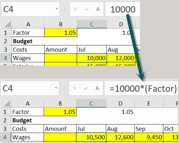
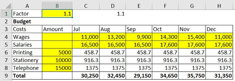
Changing cell B1 (Factor) will now update all the cells as per Figure 11.
Make sure you select the Formulas option as per Figure 8 to preserve formatting when you Paste. If you don’t click the Formulas option, then the format of the copied cell (D1) will also be applied to the selected range C4:H8.
3. Is there a formula to find the last used cell in a column?
Answer: The solution in 2005 was an array formula. Array formulas require a special entry. You type the formula and then press Ctrl + Shift + Enter. If you are in an older Excel version, you still must use that special entry. In the current version you can just enter the formula as per normal.
Let’s assume we are testing column A. This formula can’t be used in column A. To find the cell reference of the last used cell in column A, use this formula. In older Excel versions you will have to use Ctrl + Shift + Enter.
=ADDRESS(MAX(ROW(A:A)*NOT(ISBLANK(A:A))),COLUMN(A1))
This displays the fixed or absolute cell reference of the last used cell including both $ signs.
ROW(A:A)*NOT(ISBLANK(A:A))
This part of the formula is within the MAX function. It calculates all the row numbers of all the cells with entries. The MAX function then returns the highest row number of all these cells.
The ADDRESS function requires a row number, which is provided by the MAX function. The ADDRESS function also requires a column number, which is supplied by the COLUMN function.
To see the value in the last cell, use the formula below. Again, older versions will need to use Ctrl + Shift+ Enter.
=INDIRECT(ADDRESS(MAX(ROW(A:A)*NOT(ISBLANK(A:A))),COLUMN(A1)))
The INDIRECT function converts a string of a cell reference into a real cell reference. It will display the entry in the last cell.

