Loading component...
At a glance
Power Query allows you to easily import data into Excel. During the importation process you can perform data cleansing operations so that the data is ready to use in PivotTables, PowerPivot or formula-based reports.
Unfortunately, Power Query does not have any inbuilt interaction features that allow the user to interact with an existing query. In past articles I've shared a technique where you can use a parameter table to interact with the query.
This article covers a technique that uses a range to interact with a query. Range names are easy to create and import into Power Query.
Worked example
This example imports sales data from a CSV file. Figure 1 shows the data set.

The goal is to only import the sales data for the state chosen by the user.
Staging query
A useful concept to embrace in Power Query is the idea of a staging query. A staging query imports the data in full. It performs all the required data cleansing operations like fixing dates, populating blanks and removing any leading or trailing spaces. It also defines the data types for all the columns. Data types define the type of data in each column.
A staging query includes all the columns that could be required by future queries. The staging query is loaded as a connection only query. This means that the query doesn't populate a table on the spreadsheet. The data is kept in the computer’s memory, rather than in a table on a sheet.
A single staging query brings the data into Excel and other queries use its output and perform data manipulations like adding/removing columns and filtering.
To create the staging query, follow these steps.
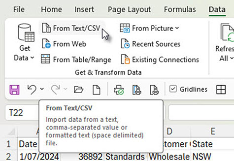
1. In a new workbook click the From Text/CSV icon on the Data ribbon.
2. Navigate to the Sales_Data CSV file. Select it and click the Import button – see Figure 3.
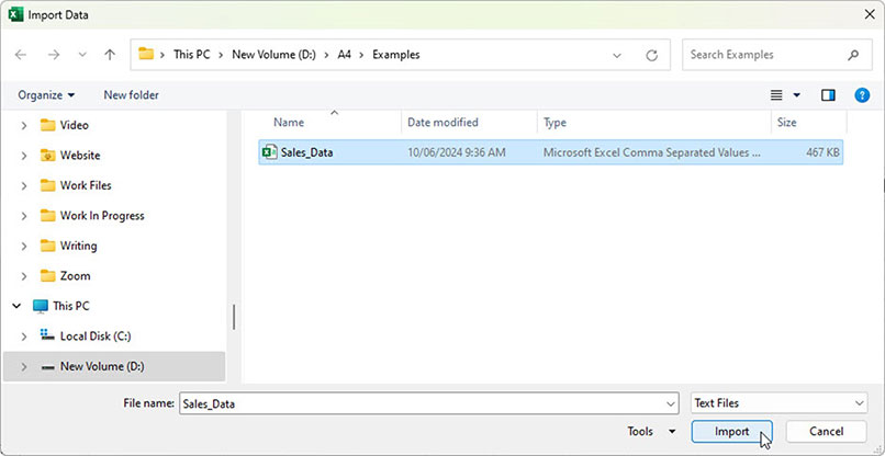
3. In the dialog that opens click the Transform Data button. This will open the Power Query window.
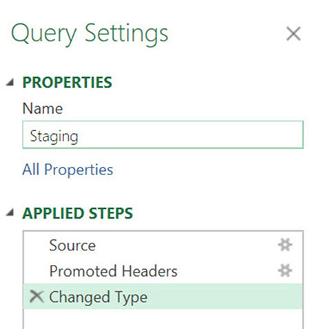
4. On the right of screen change the name from the file name to Staging – see Figure 4.
At this point any data cleansing fixes would be performed and captured as steps in the Query. This data does not require any fixing and is ready to capture.
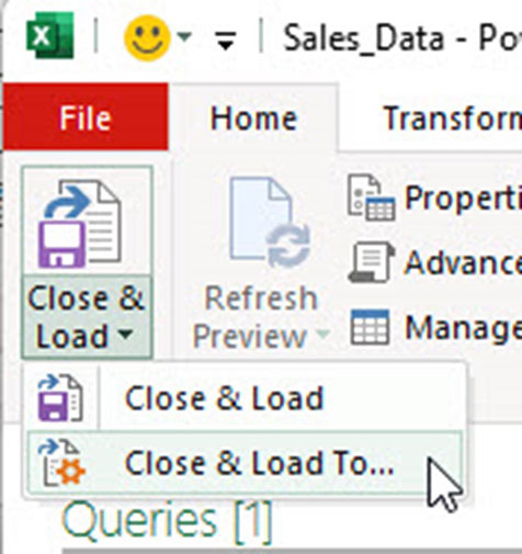
5. On the left of the Home ribbon, click the drop down on the Close & Load icon and choose Close & Load To – as per Figure 5.
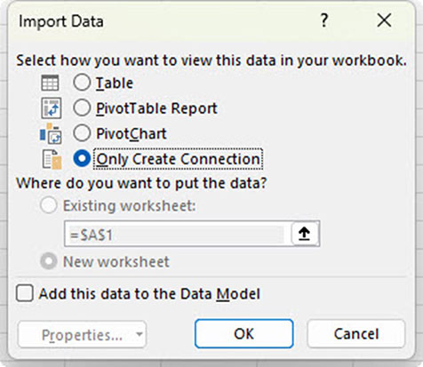
6. Select the Only Create Connection option and click OK – see Figure 6. This saves the table into memory, rather than to a sheet.
The next query captures the states in the data to use in a drop-down list for the user to select a state.
States list query
To create a list of the states we will reference the Staging query. Referencing means taking the output of one query and using it as the source for a new query.
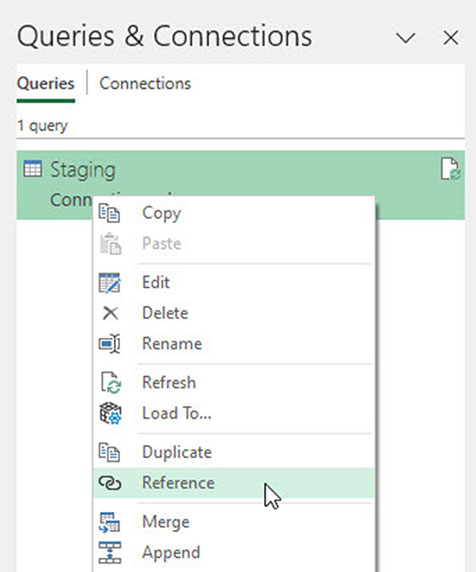
On the right of screen right-click the Staging query and choose Reference – Figure 7.
This opens the Power Query window.
Change the query name on the right to tblStates.
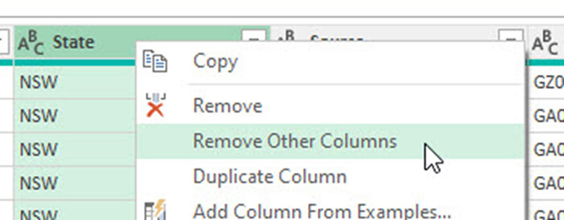
Right-click the State column header row and choose Remove Other Columns – see Figure 8. This leaves the State column as the only column in the data.
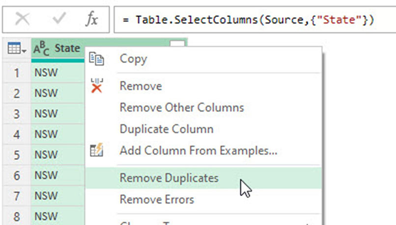
Right-click the State column header row and choose Remove Duplicates – see Figure 9.
This creates a list of unique states – see Figure 10.
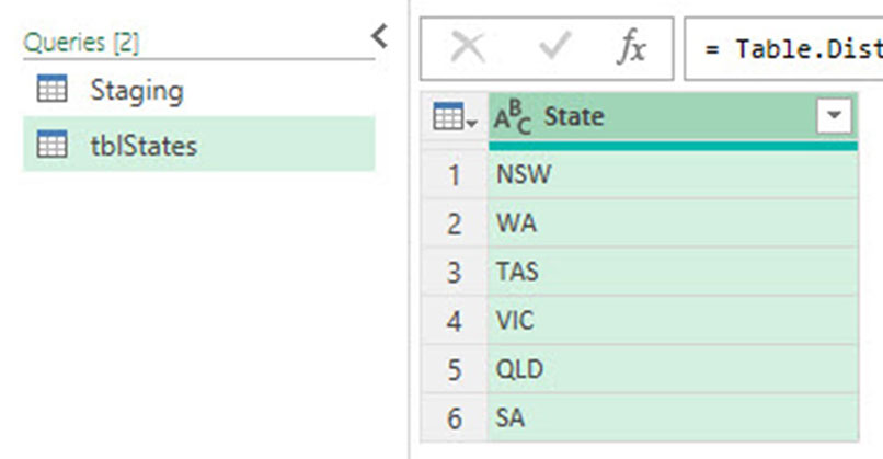
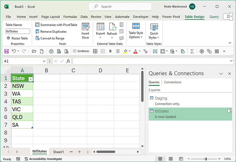
Click the Close & Load icon to populate a table on a new sheet - see Figure 11.
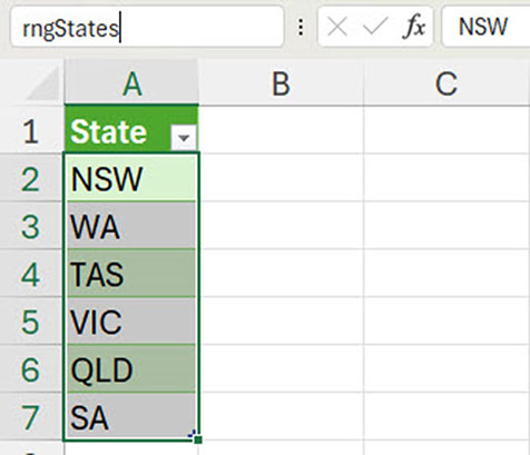
In the new sheet, select the range A2:A7 and click in the Name Box (left of the Formula Bar) and type rngStates and press Enter – see Figure 12.
This has created a range name called rngStates that refers to the states listed in the table created by the query. This named range will update if the table changes.
The range name can be used to populate a drop-down list of states.
In a blank sheet in the same file enter Select State in cell A2.
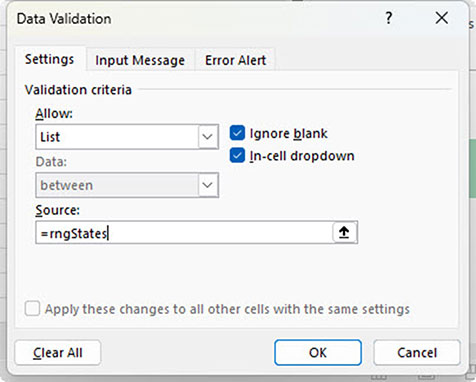
Select cell B2 and press, in sequence, the keys Alt D L. This opens the Data Validation dialog.
In the Allow: drop down select List.
Click in the Source: box type =rngStates and click OK – see Figure 13.
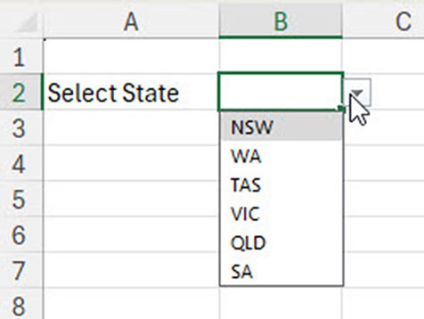
This has created a drop-down list in cell B2 – see Figure 14.
Select cell B2 and choose a state. Click in the Name Box and type StateFilter and press Enter.
Filter Query
On the right of screen, right-click the Staging query and choose Reference.
Rename the new query to SalesData. This query imports just the state sales.
Click the filter drop-down in the State header row and choose NSW. Click the Close & Load to import only the NSW data.
This query needs to be edited to add in the user interaction.
Adding user interaction
We can capture and use the entry in cell B2 in the final query.
Select cell B2. In the Data ribbon click the From Table/Range icon.
The query will be named the same as the range name.
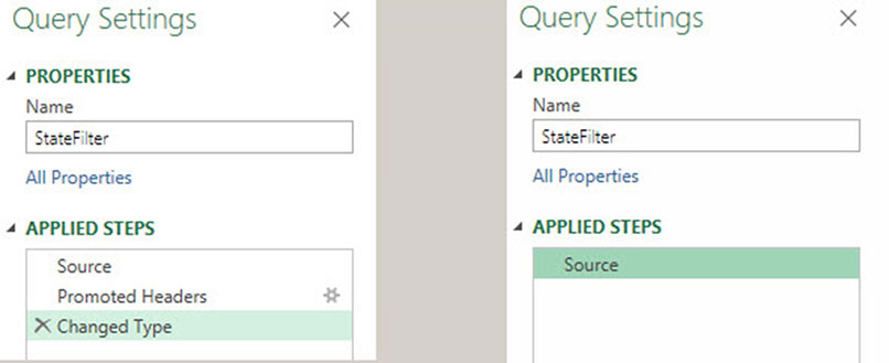
It will have two steps added that we don’t need. Delete the last two steps using the cross on the left of the step name to leave just the Source step – see Figure 15.
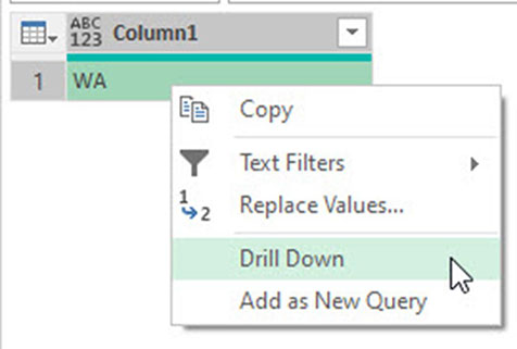
Right-click the chosen state and choose Drill Down - see Figure 16.
This captures the selected state.
Click the Close & Load icon drop down and Select the Only Create Connection option and click OK.
Double-click the SalesData query in the Queries & Connection task pane on the right of screen.
Select the last step called Filtered Rows.
In the Formula Bar replace "NSW" with StateFilter. If you can’t see the Formula Bar, click the View ribbon and tick the Formula Bar check box (top left).
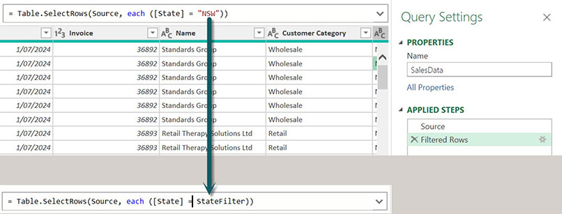
Click Close & Load to update the queries.
In the sheet with the state drop-down choose a different state.
Press Ctrl + Alt + F5 to refresh all the queries. The SalesData sheet will be updated.
Range names are an easy way to add user interaction to a Power Query.
Adding user interaction makes delegation simpler as the user only needs to update cell entries and not edit queries.

