Excel tips: how to use Power Query date tables

In my December 2016 article “The dating game”, I discussed the advantages of using an Excel-based date table in your PivotTable reports. These are especially helpful with reporting on the Australian financial year. Power Query can also create date tables. The Power Query technique is flexible and can be applied to any financial year.

In my July 2018 article “How to harness Power Query in Excel”, I demonstrated how to use a parameter table to allow the user to interact with a Power Query without having to edit the query. That technique required a separate Query for each input parameter.

This technique uses range names to interact with a Power Query. This article is more advanced than previous Power Query articles as it uses numerous M language commands, the underlying language of Power Query. The companion video will go into more detail about aspects of this technique.

Parameter table

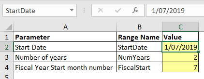
The parameter table is shown in Figure 01. 

Rows 2 and 3 are self-explanatory. Row 4 is the month number of the first month of the required financial year. The Australian financial year begins in July, so we enter 7. You would enter 4 for an April to March financial year.

Column C has three input cells (yellow). Each input cell has been named. The name used is in column B. Cell C2 is named StartDate. To create a named cell, select the cell and click in the Name Box (top left corner of Figure 01), type the name and press Enter. The name can’t start with a number or contain a space. You can use the underscore character to separate multiple words in a name, e.g. Start_Date.

The following instructions and screenshots are based on Excel 2016 and later versions. If you have the Power Query add-in for an earlier version, you can also do this, but the screens and icons may vary.

Creating the query

1. Click on the Data ribbon tab. Click the Get Data dropdown (far left), select the From Other Sources option and choose Blank Query (bottom of list).

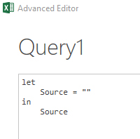
2. In the Power Query window that opens, on the Home ribbon, click the Advanced Editor icon. The editor with a blank query is shown in Figure 02.

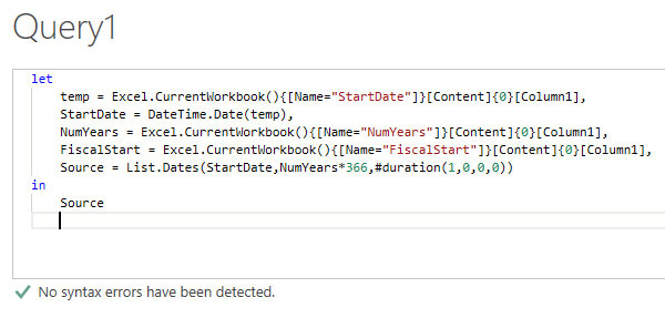
3. Click to the right of the let statement, press Enter and then the Tab key. Type the following line of code and press Enter. Refer to Figure 03 to see the completed code.

temp = Excel.CurrentWorkbook() {[Name=”StartDate”]}[Content]{0}[Column1],

Note: Power Query is case-sensitive, so make sure you match the case of the words used. There are also three different bracket types used in this line, so make sure you use the correct ones. Don’t miss the comma at the end.

The above line captures the entry in cell C2 by referring to the StartDate range name. Power Query treats the range name like a single column table with one entry. The 0 refers to the first entry in Column 1, which is the date entered. In Power Query, the index number on columns starts at zero. This is not intuitive, and needs to be understood and remembered. Index number 1 extracts the second entry from a column – not applicable in this case.

4. The next line of code is StartDate = DateTime.Date(temp), This line uses another variable called StartDate to convert the temp variable value into a Date type.

In most cases when you are using dates in Power Query, you must make sure the value is a Date data type. The entry in the temp variable is a DateTime data type. DateTime and Date are two different data types. Using the wrong data type can cause queries to fail. There should be a green tick at the bottom of the dialog. To ensure this has worked correctly, click Done. Click on the temp step (right of screen) and the StartDate step, and make sure there are dates showing below the Formula Bar (left of screen).

5. We need to add two more lines to capture two more variables. Click the Advanced Editor icon again. You can copy the temp line from above and modify it to create these two new lines. You can use Ctrl + C and Ctrl+ V. You need to replace the variable name (first word in the line) and the range name between the quotation marks. On each of these two new lines, the variable name is the same as the range name. See Figure 03 for the code so far. The first Source line in Figure 03 has been amended to Source = List.

Dates(StartDate,NumYears*366,#duration(1,0,0,0))

Note: there is no comma on the end of this line as it is the end of the query. This line uses two of the variables from above with the List.Dates function to create our list of dates.

The first argument in the List.Dates function requires a Date data type. The second part is the number of periods required – in this case, days. We multiply by 366 to ensure we include leap years. The #duration command on the end instructs the List.Dates function to return a list of days. To complete the query, return to the Power Query window. There should be a green tick at the bottom of the Advanced Editor dialog. Click Done.

6. A list of dates is shown. Note: in Power Query, a list is not a table – we need to convert it into a table. Click the Transform tab. On the left, click the To Table icon. You can also right-click the List column header and choose To Table. A dialog will open. Click OK to accept the default options.

7. Double-click the Column 1 heading. Rename it to Date.

8. Click the icon on the left of the column heading and choose Date.

I will demonstrate a technique that allows us to include financial years, quarters and months numbers:

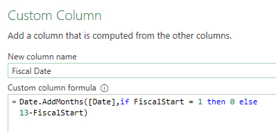
9. Click the Add Column tab. Click the Custom Column icon. Change the name to Fiscal Date and enter the following formula as per Figure 04.

=Date.AddMonths([Date],if FiscalStart = 1 then 0 else 13-FiscalStart)

In the case of the Australian financial year, 7 is subtracted from 13, which adds six months to the Date. 1/7/2019 is converted to 1/1/2020. Subtracting from 13 doesn’t work if your financial year is the same as the calendar year.

The if statement handles that difference by adding zero months to the date. This is a temporary column and will eventually be removed.

10. We will add extra columns based on the new Fiscal Date column.

11. Select the Fiscal Date column; click the Add Column tab. There is a Date icon drop-down on the far right. Click on it, choose Year and then Year.

12. Select the Fiscal Date column again, use the Date dropdown, choose Quarter and then Quarter of the year.

13. Select the Fiscal Date column again, use the Date drop-down and choose Month, and then Month.

14. Right-click the Fiscal Date column and choose Remove.

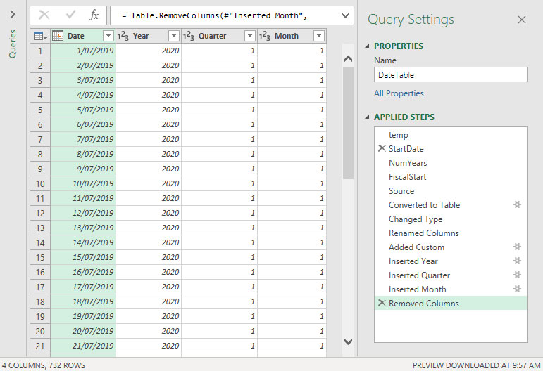
15. Rename the query to DateTable in the Name box, and on the Home Ribbon, click Close & Load. The final query is shown in Figure 05.

16. After changing the entries in the yellow cells in the parameter table (Figure 01), you can right-click the date table and choose Refresh to update the table.

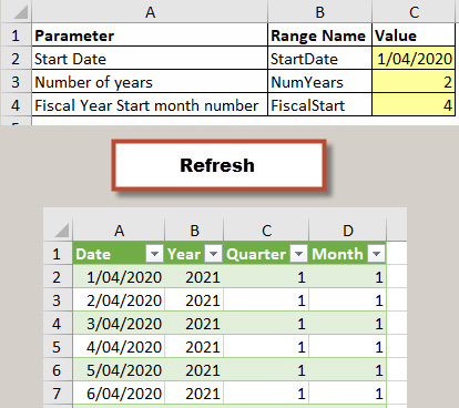
Figure 06 shows changes in the parameters and the refreshed date table.

The companion video and Excel files (blank & complete) will go into more detail to demonstrate these techniques.

Neale Blackwood CPA runs A4 Accounting, providing Excel training, webinars and consulting services to organisations around Australia. Questions can be sent to [email protected]