Record school holidays in an Excel date table

Date tables are a powerful way to include extra information in your date-based reports. A date table allows you to identify specific characteristics for each day. Identifying public and school holidays could make your sales forecasts more accurate.

Public holidays only require you to identify individual dates; school holidays are more of a challenge as they involve date ranges. 

This technique can be applied to situations where you need to identify date ranges and individual dates. For example, you might need to schedule plant shutdowns for maintenance or upgrades. 

Formatted tables

This technique uses Excel’s Formatted Table feature. The examples will demonstrate their use, flexibility and scalability. The Format as Table icon is on the Home ribbon. Using it on a table instructs Excel to treat the table like a simple database. The main advantage of formatted tables is that they automatically expand to include extra rows and columns.

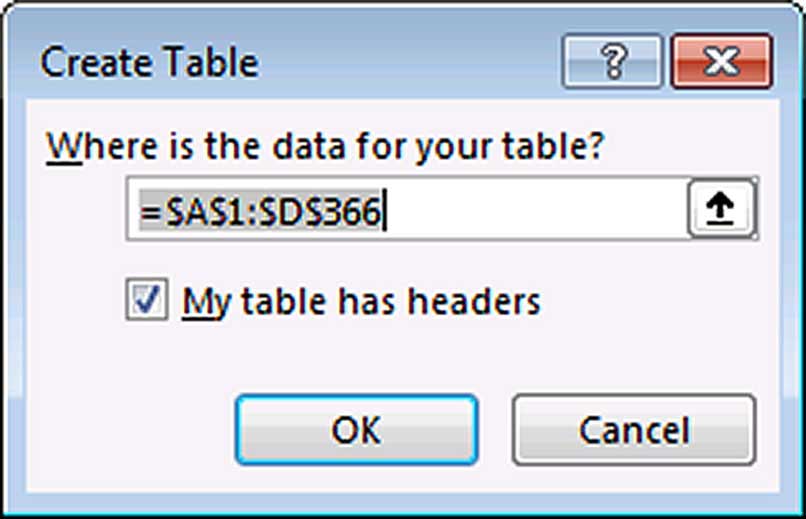
To create a formatted table, make sure your table has no blank rows, no blank columns and your headings are bold. This ensures Excel will correctly estimate the table range. Select a cell in the table and press Ctrl + T to apply Format as Table with the default blue colour. The dialog in Figure 1 displays.

Ensure the “My table has headers” option is ticked and click OK. 

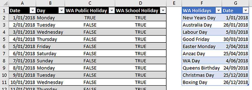
I will use three formatted tables. The first two are shown in Figure 2 (below). The public holiday dates are for 2018 and WA. 

On the left of Figure 2 is the date table. I’ve named it tblDates. Excel gives each formatted table a unique generic name, for example, Table1. 

When a formatted table is selected, a Design ribbon tab is displayed. On the far left of the ribbon you can provide a more meaningful name. I recommend using a tbl prefix for all formatted tables. This helps identify it as a formatted table. If you use range names this distinction is useful. 

Table names can also be used in formulas. If you use the prefix, then when you type tbl in a formula you will see a list of all the formatted tables in the file. You can use the Design ribbon to change the colour and other options for the formatted table.

Column A is used to list all the dates required for your file.

On the right of Figure 2 is the public holiday table. It is named tblPublicHols. 

You can have multiple formatted tables in the same sheet. Always ensure there is a blank column between the tables. This makes it easier to identify, select and work with the tables. 

I use a dedicated sheet to hold these type of lookup tables. Transactional (longer) data tables, I prefer to have in separate sheets. 

The public holiday table is simple and contains only date entries. You could include multiple years in this table. The name of the holiday is not required but it is useful to ensure you haven’t missed a public holiday.

The date table has formulas in columns B, C and D. When you enter a formula in a column in a formatted table, the formula automatically copies to all the other cells in that column. 

The formula for cell B2 is: 

=TEXT([@Date],"dddd")

The TEXT function creates text from a value, in this case a date, based on a custom format. 

The [@Date] section of the formula is part of the formatted table functionality. The square brackets surround the column name and the @ symbol refers to the same row in the current table. This is called a Structured Reference, however I will refer to them as table names as it more descriptive. 

The custom format must be enclosed in quotation marks. The "dddd" in the formula instructs Excel to show the full day name of the date. The TEXT function is frequently used to automate dates in report headings. 

You could use a cell reference instead of the table name as below: 

=TEXT(A2,"dddd")

The formula in cell C2 is:

=COUNTIFS(tblPublicHols[Date],[@Date])>0

The COUNTIFS function counts how many times an item appears in a range. The reference to tblPublicHols[Date] refers to the Date column in the tblPublicHols formatted table. The [@Date] reference is to the Date column in the same row in the date table.

If a date doesn’t appear in the tblPublicHols column range, the COUNTIFS function will return 0. By comparing the result of the COUNTIFS function with 0, we can identify if a date is a public holiday. 

If the date is counted, then TRUE is returned, otherwise FALSE is displayed. 

If you would prefer to display text instead of TRUE and FALSE, then you could use a formula like:

=IF(COUNTIFS(tblPublicHols[Date],
[@Date])>0,"Yes","No")

This will return Yes if the date is a public holiday and No if it isn’t.

School holidays

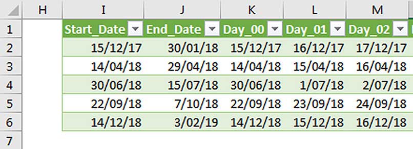
The structure of the school holiday table (named tblSchoolHols) has two input columns, Start_Date and End_Date. The remaining columns calculate the individual dates of the school holiday. The layout of the school holiday table is shown in Figure 3 (below). 

The Day columns contain formulas and continue to the right until Day_56. You need as many columns as there could be days in the date ranges. Creating the Day headings is easy. Dragging cell K1 across with the Fill Handle (small black cross, bottom right-hand corner of cell) will automatically increment the number. 

The formula in cell K2 is: 

=IF($I2+RIGHT(K$1,2)*1<=$J2,$I2
+RIGHT(K$1,2)*1,"")

I have used cell references rather than table names to shorten the formula and to make it easier to explain. 

The important part of this formula is +RIGHT(K$1,2)*1 

The RIGHT function extracts text characters from the right of a cell. In this case, the two characters extracted are 00. The text 00 is multiplied by 1. Multiplying text numbers by 1 converts them into real numbers. This, combined with the headings, provides a sequential number as we copy it across. 

We add that sequential number to the start date from cell I2 to increment the date and compare the new date with the end date in J2. If the new date is less than or equal to the end date, we display the new date, otherwise we display a blank cell using "". 

The Day number headings enable the formula to increment the date as the formula is copied across. 

This formula can be copied across to all the other Day columns. You should use copy and paste and not the Fill Handle to copy the formula. The Day columns include each school holiday date for the five school holiday periods.

Copy warning

If you use table names such as [@Date] or tblPublicHols[Date] in your formula and try to copy the formula across a table with the Fill Handle, then you will encounter two issues: the formula doesn’t automatically copy down the whole column; and the column name references change like relative references. 

In general, don’t use the Fill Handle to copy across formulas containing column-based table names. Using copy and paste works. In the companion video on intheblack.com, I will share workarounds for the Fill Handle copy-across issue. 

Date table

We can use the COUNTIFS function again to determine if a date is a school holiday. In the date table (Figure 2) the formula that identifies school holidays in cell D2 is:

=COUNTIFS(tblSchoolHols[[Day_00]:
[Day_56]],[@Date])>0

The table column names allow you to create a large range reference by using a start column [Day_00] and an end column [Day_56] separated by a colon. This formula displays TRUE if a date is a school holiday and FALSE if not. If, instead, you want to display Yes or No in column D, you would use:

=IF(COUNTIFS(tblSchoolHols[[Day_00]:
[Day_56]],[@Date])>0,"Yes","No")

This date table enables you to analyse date-based transactional data with public and school holiday dates.

Excel 2013 and later versions have a Relationships option in the Data ribbon. You can relate two tables much like a relational database, so that you can report on multiple tables in a single PivotTable.

The companion video and Excel files (blank and complete) will go into more detail to demonstrate these techniques.

Neale Blackwood CPA runs A4 Accounting, providing Excel training, webinars and consulting services to organisations around Australia. Questions can be sent to [email protected]