Loading component...
At a glance
Power Query allows you to extract data from multiple sources and perform data cleansing operations on that data. I wrote about Power Query in the June 2016 and August 2017 editions of INTHEBLACK.
In Excel 2010 and Excel 2013, Power Query is available as a free add-in from Microsoft. In Excel 2016, Power Query is called “Get & Transform” and can be found in the Data ribbon.
One of Power Query’s current limitations is that there isn’t a built-in mechanism to allow the user to interact with the query. Instead, to make changes, you must edit the query. This can be daunting for most users and makes it difficult to supply standalone interactive solutions. However, there is a workaround. The Format as Table icon on the Home ribbon allows you to define a table that Excel will treat like a basic database.
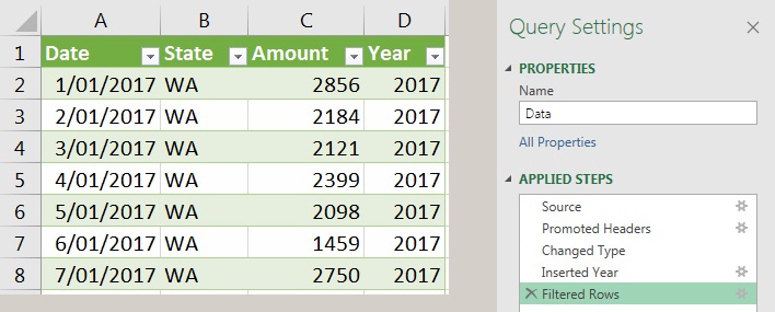
The technique I will demonstrate uses a parameter table. The data used in the example (see Figure 1) is simple, but the technique can be applied to more advanced solutions. Although this technique is rather advanced, it requires the least amount of query code editing to achieve interaction.
Demonstration
I will briefly outline the steps to importing a CSV file using Power Query (for more detail, access the above-mentioned articles). I will then focus on how to use the parameter table to modify the query and allow the user to interact with it.
Importing (Excel 2016)
- Click on the Data ribbon tab, then on the Get Data dropdown. Choose From File and next choose From Text/CSV.
- Navigate to the location of the Data.csv file, click the file, then click the Import button.
- Click the Edit button at the bottom of the dialog.
- The Power Query window will open, with the data displayed. This window is separate to Excel.
- Right-click the Date column. Choose Change Type and select Date.
- You will need to add a Year column to make it easier to control the year to import. Click on the Date column and then on the Add Column ribbon tab. Click the Date icon dropdown and select Year. This adds a new column named Year.
- Right-click the Year column heading. Choose Change Type and select Whole Number.
- Use the filter icons to filter the State column to WA and the Year column to 2017.
- The importation steps are complete. On the Home ribbon, click the Close and Load icon to upload the data to a sheet within the file. I have named this sheet Extract.
The resulting table and the query’s Applied Steps are shown in Figure 1.
Power Query will repeat the Applied Steps (listed left) in sequence each time the data is refreshed.
Step 8 equates to the Filtered Rows highlighted in Figure 1. This is the step we will modify to allow user interaction with the query.

The parameter table allows a user to select a state and a year to use as the filters in the importation process.
Formatted tables
Formatted tables were added in Excel 2007. The Format as Table icon on the Home ribbon allows you to define a table that Excel will treat like a basic database. There are many advantages to using formatted tables that I mention during the companion video to this article. One is that they work seamlessly with Power Query.
Creating a formatted table is as easy as selecting a cell in the table and pressing Ctrl + T, then pressing Enter. This applies the default blue colour. At this point, Excel will guess the data range. It will calculate the range correctly, provided you have a bold headings row and no blank rows or blank columns in the table.
Once created, you can rename the table. When the table is selected, a Design ribbon tab is displayed and you can change the name on the far left-hand side of the ribbon. I use tbl as a prefix on my table names, so as not to confuse them with range names.
Parameter table

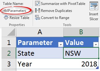
I have used Format as Table and created the parameter table shown in Figure 2. It is named tblParameters. It only has two parameters, but you can add as many as you require and the table will automatically expand to include them (another advantage of formatted tables).
We will now create two new queries; one for each parameter in the table.
- Select a cell within the parameter table. Click the Data ribbon and then the From Table/ Range icon. This opens the Power Query window.
- Rename the query to State in the Query Settings section on the right of screen.
- Click the filter icon on the Parameter column and filter by State.
- Right-click the Value column heading and choose Remove Other columns.
- Right-click the Value column heading. Select Change Type and choose Text.
- Right-click the NSW entry and choose Drill Down. This converts the query from a table into a single entry that represents the state entered in the parameter table.
- On the Home ribbon, click the dropdown on the Close and Load icon, and choose Only Create Connection. Click OK.
Repeat steps 1 to 7 with the following changes for Year.
- In step 2, rename the query to Year.
- In step 3, filter the Parameter column by Year.
- For step 5, change the Value column type to Whole Number.
- In step 6, right-click the entry 2018 and choose Drill Down.
The State and Year queries are now like variables, as they return a single entry. We can insert the query names into the initial query filter formula to make it interactive.
Inserting parameters
Return to the Extract sheet and select a cell in the table. Click the Query ribbon tab and click Edit.
Select the last step as highlighted in Figure 1.

In the Formula Bar situated below the ribbon, we need to make the following changes. Replace WA with State and 2017 with Year. See Figure 3.
If the Formula Bar isn’t visible, click the View ribbon and tick the Formula Bar option.
On the Home ribbon, click the Close and Load icon to capture query changes. Any changes the user makes in the parameter table will be automatically updated in the Extract sheet when the query is refreshed.
You can add more parameters to the table. Each one will require its own query to extract the parameter value. Use the same seven steps and a descriptive name for the query.
Column data types (step 5 of 7) are important in Power Query. The data type needs to match the data type of the column being filtered or modified in the imported data. This is especially important for date columns.
The companion video and Excel files (Data and Power Query Parameters) will go into more detail to demonstrate these techniques.
Neale Blackwood CPA runs A4 Accounting, providing Excel training, webinars and consulting services to organisations around Australia. Questions can be sent to [email protected]

