Excel tips: importing share prices into Excel

The Data Types feature imports share prices and other share-related information using stock exchange and stock (ticker) codes. 

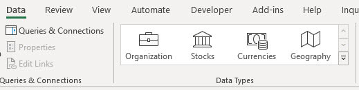
You can check if you have access to Data Types by clicking the Data tab in the Ribbon, as shown in Figure 1. You will need an internet connection for Data Types to update.

Getting started

1. In a blank sheet, enter Stock in cell A1. In cell A2, enter xasx:wbc. XASX is the Australian Stock Exchange code and WBC is the stock (ticker) code for Westpac Banking Corporation. 

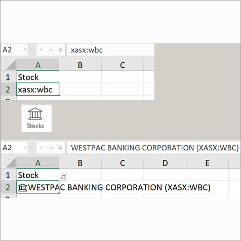
2. Select cell A2, click the Data ribbon and click the Stocks icon in the Data Types section. The entry will convert as shown in Figure 2. 

3. Widen column A to fit the text. Copy cell A2 to A3 and A4. In cell A3, enter xasx:cba. In cell A4, enter xasx:anz. These are the codes for Commonwealth Bank and ANZ Bank, respectively.

4. Select A1:A4, press Ctrl + T and then press Enter to convert the range into a formatted table.

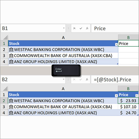
5. To see something amazing, enter Price into cell B1 and press Enter – see Figure 3.

The table expands to include the new column, which is standard for formatted tables. What isn’t standard is that the Price field automatically populates with a formula and values. 

Note the formula in the Formula Bar in cell B2 at the bottom half of Figure 3. This is part of the Data Type functionality where the full stop is used to access the fields within a Data Type.

DISCLAIMER

Excel provides a disclaimer above the Formula Bar that appears when using the Stocks feature. This warns that the information is provided as-is and is not meant for professional or trading purposes or advice.

Different currencies

1. In cell C1, enter Currency. 

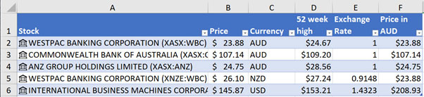
2. In cell A5, enter xnze:wbc. In cell A6, enter xnys:ibm. These two stocks are from different stock exchanges – New Zealand and New York, respectively. They will update with their name, price and currency.

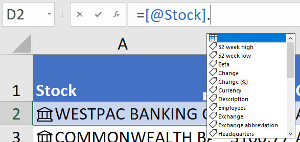
3. In cell D2, enter = and use the mouse to select cell A2 and press the full stop. The list of available fields will display as a dropdown – see Figure 4. Select “52 week high” and press Enter. Rename the column to 52 week high.

Exchange rates

1. As a companion for the stock codes, there are also exchange rate codes (see Figure 1).

2. In a separate, blank worksheet enter Exchange Rates in cell A1.

3. In cell A2, enter NZD/AUD. In cell A3, enter USD/AUD. Select A1:A3, press Ctrl + T and press Enter.

4. Select A2:A3, click the Data tab and click the Currency icon. 

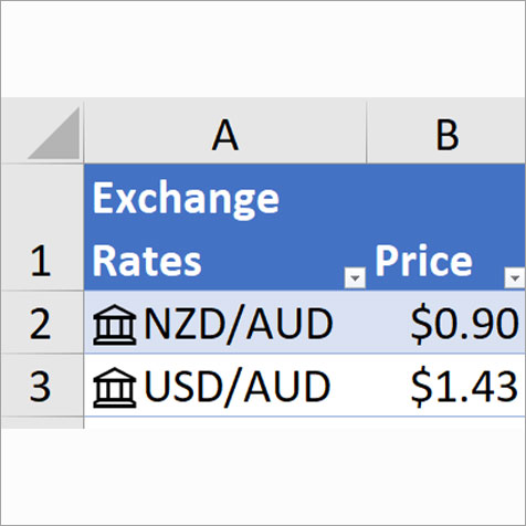
5. Enter Price in cell B1. The table will update as shown in Figure 5.

The Accounting number format applies automatically to the Price (see Figure 3). This format places the $ sign in the left of the cell.

I prefer to use the Currency number format, which places the $ sign next to the number as per Figure 5. Although only two decimal places are displayed, the exchange rate has four decimal places.

To make this table easier to look up, we can add a code for the currency that is being converted to AUD. This assumes all the codes we list in this table will be converting to AUD. 

6. Enter Code in cell C1. 

7. Enter the following formula in cell C2:

=LEFT([@[Exchange Rates]].[Ticker symbol],3)

8. The ticker symbol field for the NZD/AUD conversion is NZDAUD. The above formula extracts the first three characters from the ticker symbol field. 

9. Since the first table has multiple currencies, we can now standardise the values and convert all the Prices to AUD using our second table. 

10. I will name the Exchange Rate table tblRates. You can do this in the Table Design tab (far left) when the table is selected. I use a prefix of tbl for formatted tables, so they list together when I type tbl in formulas. It also tells me the name is for a formatted table rather than a range name.

11. In our first table, enter Exchange Rate in cell E1. In cell E2, to extract the exchange rate from the other table, enter the following formula:

=IF([@Currency]="AUD",1,XLOOKUP([@Currency],tblRates[Code],tblRates[Price],0))

12. The IF function returns 1 if the currency is AUD. The XLOOKUP function will extract the rate from the exchange rate table if it finds the currency code. It will return zero if the Currency code cannot be found. If a new currency code appears in the first table, you can enter its exchange rate code in the exchange rate table to enable conversions.

13. We can add a further column to the first table. Enter Price in AUD in cell F1. In cell F2, enter the following formula:

=[@[Exchange Rate]]*[@Price]

14. If you use the mouse to select cells B2 and E2, Excel automatically enters the references with the square brackets. These are called structured references and are part of the formatted table functionality. Figure 6 shows the final table. 

Data card

You can also access the Data Types functionality outside a formatted table. In another blank worksheet in cell A1, enter xasx:wbc and define it as a Stocks Data Type via the Data Ribbon tab. In cell B1, enter the following formula:

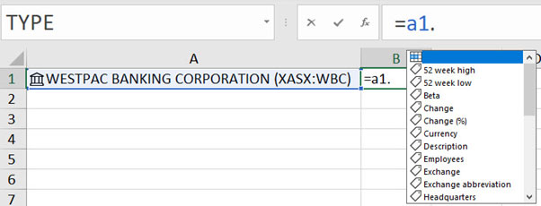
=A1.Price

When you type the full stop, you will see the available fields listed – see Figure 7.

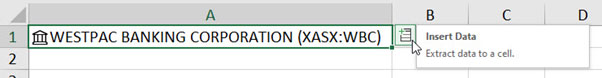
Another way to access these is via a small icon that appears to the right of the cell when you have the Data Type cell selected - see Figure 8.

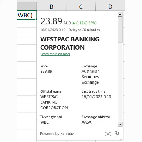
You can right click any cell that has been defined as a Data Type and select Show Data Type Card to see all information listed as shown in Figure 9.