Excel tips: how to create hyperlinked index sheets

It is best practice to use separate sheets for separate sections of your Excel file. This means you should have separate sheets for instructions, inputs, data, reports, dashboards, validations and workings.

This can lead to a lot of sheets, and the more sheets you have, the harder it is to navigate between them all.

In these situations, it is useful to have an index sheet, with hyperlinks to all other sheets, to speed up and simplify navigation around the file. On each sheet, you can also have a hyperlink back to the index sheet.

Creating a hyperlink is a manual process that takes a few clicks, and manual hyperlinks can break if the sheet name changes.

I will share a way to create a flexible index sheet, starting with non-hyperlink solutions.

Link hack

Creating a formula that links to another sheet is quick and easy. Combine that with a keyboard shortcut, and you have a robust alternative to hyperlinks.

With a cell selected that links to another sheet, or another cell in the current sheet, you can press Ctrl + [ to jump to that cell. To return, you press the F5 function key, then press Enter.

This return shortcut also works for the hyperlinks that follow. These shortcuts are also useful when reviewing formulas.

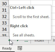
You can right-click the navigation arrows on the left on the sheet tabs at the bottom, left of the Excel screen, as shown in Figure 1.

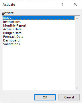
When you right-click, a list of all the sheets is displayed, as seen in Figure 2.

In older versions of Excel, the list may only show the first 10 sheets.

Formula-based hyperlinks

You can create flexible hyperlinks using inputs and the HYPERLINK function. This function can be applied elsewhere to include hyperlinks with instructions and standard procedures.

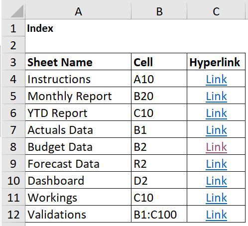
The HYPERLINK function is not easy to use, but it can be simplified with a trick. Figure 3 has a table we will use to create an index sheet for a file.

Columns A and B have data entries. If a sheet name changes, you need to update the name in column A. Changing either the sheet name or the cell reference adjusts the hyperlink destination in column C.

As you can see from row 12, you can even create a hyperlink to a range. Column C contains the HYPERLINK function.

The formula in cell C4, which has been copied down, is:

=HYPERLINK(“#’”&A4&”’!”&B4,”Link”)

The # symbol at the front is the trick to making this work. This symbol makes the sheet or cell reference easier to create.

The HYPERLINK function in cell C4 requires the following text string in its first argument to create the hyperlink: 

#’Instructions’!A10

The single inverted commas must enclose any sheet name that includes a space.

The text in the second argument of the HYPERLINK function has the text that is displayed in the cell. The text will be automatically underlined like a normal hyperlink.

Being able to specify the sheet name and the cell or range reference gives you the flexibility to link to anywhere in the file.

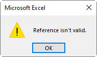
If you specify a hidden sheet name, nothing happens when you click the hyperlink. If the sheet name is wrong, then the error message in Figure 4 displays.

Sheet name changes

You can extract a sheet name using a formula. Instead of typing the name in the index sheet, you have a couple of options.

You could create a formula in the destination sheet that extracts the sheet name formula. You can then link to that cell from the index sheet. When the name changes, the formula automatically updates the index sheet.

Alternatively, you could enter the sheet name formula in the index sheet and link to a cell in the destination sheet. This will extract the destination sheet name. The downside of this technique is that the formula becomes quite long.

I have provided examples of both formulas later in this article.

Excel versions

In practical terms, there are currently two versions of Excel.

1. The subscription version, called Microsoft 365 or Excel 365, which has lots of new features.

2. All the older versions, which will not be updated with the new features.

Below are two versions of each of the two formulas mentioned above, one for the subscription version and one for every other version of Excel.

Destination sheet formulas

These are entered in any cell in the destination sheet. The same formula works no matter which sheet or cell you enter it into.

Subscription version

=LET(c,CELL(“filename”,A1),RIGHT(c,LEN(c)-SEARCH(“]”,c)))

All versions

=RIGHT(CELL(“filename”,A1),LEN(CELL(“filename”,A1))-SEARCH(“]”,CELL(“filename”,A1)))

Having created one formula, you can copy and paste it to the other sheets. Once these formulas are in the destination sheets, you can link to them from the index sheet. This captures the sheet name on the index sheet.

Index sheet formulas

Formulas to enter in the index sheet are the same as the ones above, but they link to another sheet, the destination sheet. In the examples below, I have used cell A1 in the instructions sheet.

Subscription versions

=LET(c,CELL(“filename”,Instructions!$A$1),RIGHT(c,LEN(c)-SEARCH(“]”,c)))

All version formula

=RIGHT(CELL(“filename”,Instructions!$A$1),LEN(CELL(“filename”,Instructions!$A$1))-SEA RCH(“]”,CELL(“filename”,Instructions!$A$1))) 

You would need to create this formula for each sheet whose name you want to automatically update in the index sheet.

Hyperlinked images

Earlier, I suggested including a hyperlink to the index sheet in all the other sheets. One way to do this is to use an image. Excel has access to many types of images in the Insert tab and the Illustrations section.

Let’s say we want to use a boomerang icon to symbolise “going back” or “returning”. We can add the icon to the sheet, right-click the icon and choose Link. This is also how you create a standard link in a cell. The keyboard shortcut to insert a Hyperlink is Ctrl + k.

As shown in Figure 5, click the Place in This Document icon on the left, choose the index sheet and click OK.

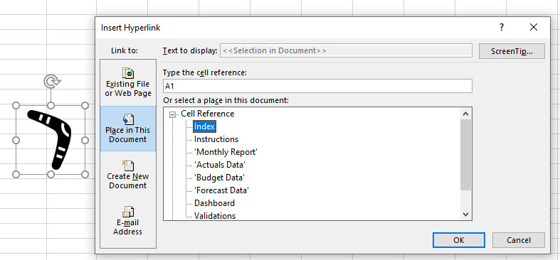
Clicking the boomerang icon will now return you to the index sheet. Once created, you can copy and paste this icon onto other sheets and the link will work. This link will break if the index sheet is renamed.

Entering a formula in every sheet

In the companion video to this article, I share a technique that can speed up destination formula entry. The technique can also be used for other tasks, and it enables you to quickly enter the same formula in the same cell in every sheet (or selected sheets) in a file.

The companion video and Excel file will go into more detail to demonstrate these techniques.

Neale Blackwood CPA runs A4 Accounting, providing Excel training, webinars and consulting services. Questions can be sent to [email protected]