Excel tips: learn data validation, paste link and zero values

I answered five questions between September and December 2004.

1. Is it possible to limit data entry in a range to unique entries only?

Excel has a built-in Data Validation feature. Unfortunately, it doesn’t offer a unique option. It does however have a Custom option that accepts formulas. We can create a formula that limits entries to unique entries.

Let’s assume we want to enter a unique code in column A.

1. Select the range A2:A100.
2. Press in sequence Alt A V V (keys not held down) this opens the Data Validation dialog. Data Validation is on the Data ribbon, right-hand side, if you want to use the icon.
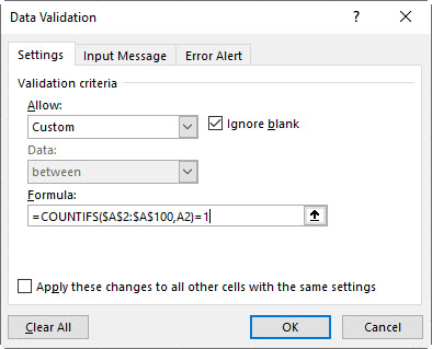
3. Select Custom from the Allow drop down.
4. Enter the following formula in the Formula box
   =COUNTIFS($A$2:$A$100,A2)=1
   See Figure 1 below for the dialog. (Question 4 below goes into more detail about COUNTIFS)

5. Click OK. 
6. That’s it. You won’t be able to enter a code twice in the range A2:A100. See below for a detailed explanation of why this works.
7. If you enter a duplicated code the following dialog will display.

8. If you want to display a more meaningful error message, then select the range again and press Alt A V V.
9. Click the Error Alert tab and create a custom message. You can have a custom Title and an Error message. Click OK. See mine in Figure 3.

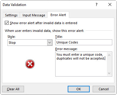
10. If you try to enter a duplicate code now the dialog that displays looks like Figure 4.

The Error message option is available for all your Data Validations not just the custom ones.

You may have noticed the Input Message tab. This allows you to create a customised message that pops up every time the cell is selected. In general, this is annoying and should only be used for inputs that happen once or twice, e.g. you send a file to someone to fill in and return. Don’t use the Input Message for cells that are entered into regularly. 

Explanation of technique

When using the Custom option for Data Validation the formula you create must return TRUE for the action you want to happen. Formula used

=COUNTIFS($A$2:$A$100,A2)=1

The COUNTIFS function counts the number of times an entry appears in a range. We compared that to 1 because we only want unique entries.

The $ signs in the formula are important. I used a fixed reference for the whole input range, but a relative reference for the cell – no $ signs. I referred to the top left cell of the range A2 in the formula. When this is applied to the other cells in the range it will change the relative reference to A3, A4 all the way down to A100. You can’t copy this data validation across to other columns.

Limitations of data validation

Unfortunately, Data Validation has two problems.

• It doesn’t stop people using Paste Special Values into a cell
• It doesn’t stop people using the Fill Handle to copy entries in the range

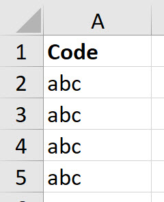
Even though I applied the above data validation I can still encounter problems, see Figure 5. 

You can use Conditional Formatting in combination with Data Validation to highlight those cells that are duplicated. This is now straight forward, back in 2004 it was more complicated.

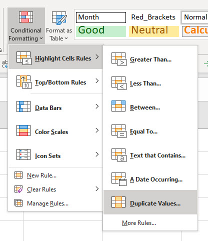
Select the range A2:A100. On the Home ribbon click the Conditional Formatting icon drop down and select the top option, Highlight Cells Rules, and then Duplicate Values as per Figure 6.

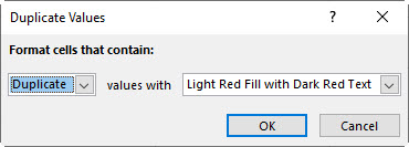
In the dialog that opens (Figure 7) you can click OK. Feel free to change the colour on the right. The default is Light Red. 

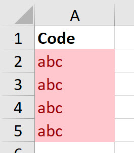
Job done, see Figure 8.

2. I use Paste Link frequently. Is there a quick way to access it instead of going through Paste Special each time?

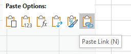
It seems like Microsoft may have read this article because now the right click menu has the Paste Link icon on it – see Figure 9 – it is the last icon in the Paste section. Now it is easy to Paste Links.

There are also keyboard shortcuts to access the Paste Options. The shortcuts below allow you to do some of the standard Paste Special pastes. All these assume you have already copied something. These keys are all pressed in sequence, not held down.

Alt H V N – Paste Link

Alt H V V – Paste Values

Alt H V A – Paste Values and number formats

Alt H V F – Paste Formulas

I use the Alt H V V shortcut all the time.

3. Is it possible to stop zero values displaying in a range?

You can use a custom number format to stop zeros displaying within a specific range.

Select the range. Press Ctrl + 1. Use the 1 on the keyboard, not the numeric keypad. This opens the Format Cells dialogue. In the Number tab select the last option, Custom.

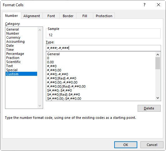
In the Type box enter the following format as per Figure 10. This format uses the comma as the thousands separator.

#,###;-#,###

Click OK.

Custom Number formats have a special layout. They can have up to four sections separated by semi-colons - see below.

Positive;Negative;Zero;Text

When you only define two sections (as we did) zeros are handled by the positive format, the first format.

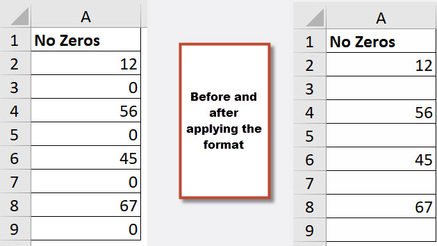
The # (hash) symbol defines a number, but it doesn’t display zeros. Figure 11 has the before and after screen shots after applying the format.

You can scroll down the Custom number list on the right of the dialog to see other built-in custom number formats. They include formats for numbers, dates, hours, minutes and seconds. 

Once you have created the new custom number format you can use it throughout the file. 

Stopping zeros displaying in the sheet

If you want to stop zeros displaying in the whole sheet you can change an Options setting. 

Click the File ribbon tab, click Options (bottom left).

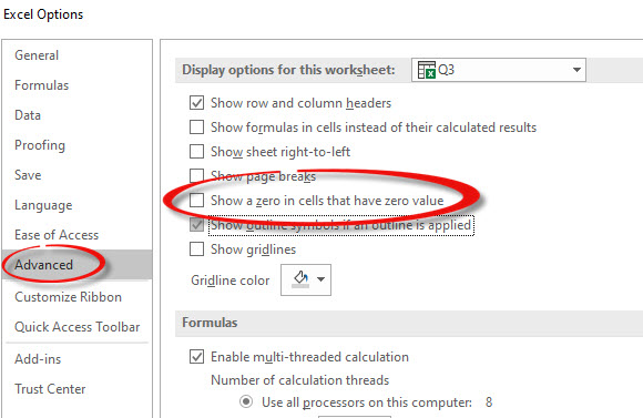
Click the Advanced option (left side) and scroll down about two-thirds of the way until you see the section shown in Figure 12. Untick the option “Show a zero in cells that have a zero value”. Click OK.

This only works for the sheet you have selected.

4. Is it possible to perform a COUNTIF based on multiple criteria?

Microsoft may have read this article too because in Excel 2007 it included a new function called COUNTIFS that allows multiple criteria counting. I used COUNTIFS in answering the first question.

The COUNTIF function counts how many times an entry appears in a range, but it is limited to one criteria.

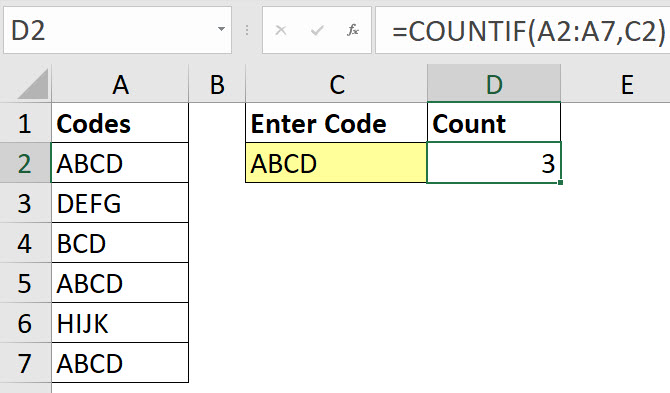
You can see an example in Figure 13.

The formula in cell D2 counts how many times ABCD appears in the range A2:A7. This is really useful if you want to see if a code exists in a range. You can use something like:

=COUNTIF(A2:A7,C2)>0

This returns TRUE if the code is in the range and FALSE if it isn’t. 

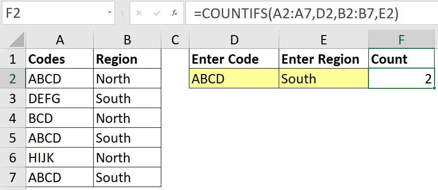
The COUNTIFS function extends the number of criteria you can look for. In Figure 14 you can see an example of a two criteria COUNTIFS.

There are two combinations of ABCD and South.

To add an extra criteria you add an extra range and an extra criteria to the end of the function arguments, all separated by commas. Each additional range needs to be “paired” with a criteria.

If you are using multiple vertical ranges their rows should correspond e.g. start and finish on the same rows. If using multiple horizontal range, then the columns should correspond e.g. each range’s starting and ending columns should be the same.

In practice the ranges tend to a fixed reference (both $ signs), especially if you need to copy and paste it. For example: 

=COUNTIFS($A$2:$A$7,D2,$B$2:$B$7,E2)

5. Is it possible to view cells’ values and formulas simultaneously?

Yes, it can be done. It is a sort of hack. You can’t see the formula and the results at the same time in the same screen but you can open two windows of the same sheet and have formulas visible in one window and the results visible on the other.

This technique comes with a warning at the bottom of the post.

It is surprising how few people know that you can display more than one window of a single file. The operating system is called Windows but over the years people have forgotten how to use multiple windows in Excel.

Multiple windows means you can have one sheet visible in one window and another sheet visible in another window so you can easily copy between the windows.

It is even better in the newer versions of Excel because you can display the windows on separate screens as well. I highly recommend dual screens. Monitors are quite cheap and the productivity savings of switching between multiple screens is worth it. My workstation has three screens.

To open a new view of the current file, click the View ribbon and click the New Window icon.

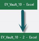
Not much changes but there is one important thing you need to notice. In Excel’s header a number has been added to end of the file name. Figure 15 has an example. Monitoring these numbers is important. Excel increments new window numbers. You can have as many windows as you need.

In the new screen to see the formulas displayed press Ctrl + ` this is the key under the Esc key – see Figure 16.

The result will look something like Figure 17.

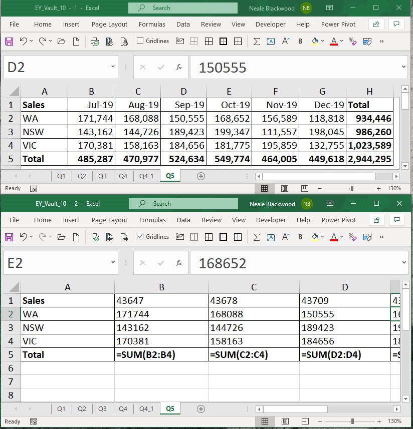
The downside of this technique is that the column widths are widened to display the formulas. 

A few things to note

• the values are displayed with no format. Row 1 has the dates, but they are now showing as numbers.
• the numbers in the top header (green) sections of each window. These numbers are important.
• The number 1 window is the main window and it should never be closed. Only close the other numbered windows. The reason is explained in the Warning section below.

Warning

This technique comes with a warning. As noted, the new window has no viewing settings, e.g. Freeze Panes is turned off and the Zoom percentage is 100%. 

Before you save the file you need to close the windows with the highest numbers first. If you save the file with more than one window visible it will retain that setting and open multiple windows. That can be confusing if someone else opens the file.  

If you close the #1 window down and save, then you will lose things like Freeze Pane settings. 

Neale Blackwood CPA runs A4 Accounting, providing Excel training, webinars and consulting services to organisations around Australia. Questions can be sent to [email protected]