Excel Tips: Three useful macros for accountants

Macros are an essential productivity tool in Excel. They can remove or reduce manual processes and speed up frequently performed tasks.

Here are three useful timesaving macros.

The companion video explains how to install and use these macros. The companion file contains the macros.

Macro Warning:

Running a macro clears Excel’s Undo list. This has two implications.

1. The macro cannot be undone.
2. Anything done before the macro was run cannot be undone.

As a precaution, save the file before running the macro. If the macro doesn’t work as expected, close the file without saving. Another option is to use a copy of the file to test the macro.

1. Fixing two PivotTable limitations

PivotTables are incredibly powerful and make it easy to create reports, but they have two limitations. Figure 1 shows both limitations.

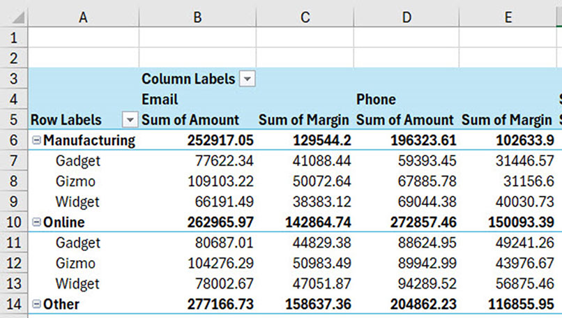
First, a new PivotTable report has no formatting applied to the values. The most common number format applied to PivotTable content is the comma format with no decimals. 

Enabling it requires about seven mouse clicks to apply to each reporting field.

The second issue is the terminology “Sum of” used in the column headings (see row 5). For presentation purposes, this terminology should be removed.

Most people don’t realise that PivotTable column headings can be amended manually. The heading name must be different to the field (column) name. The workaround is to place a space at the end of the field (column) name.

A macro may offer a full or partial solution for manual operations that need to be performed repeatedly.

In this case, a macro can fix both issues immediately. See the macro shown in Figure 2.

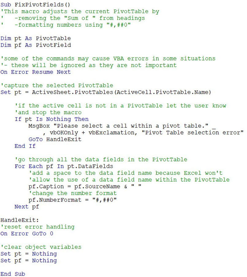
The green text is only used to document and explain the code – it doesn’t do anything.

The two Dim statements at the top create two variables, pt and pf – one for the PivotTable and one for the PivotTable field. Variables make the code shorter and easier to write.

Some of the macro code could cause an error, so the On Error Resume Next statement instructs Excel to ignore all errors and perform the next line of code. 

Use this line of code sparingly, because it can cause problems if used in the wrong situation.

To run this macro, the user must first have a cell selected in a PivotTable. The pt variable captures the PivotTable. If the user doesn’t have a PivotTable selected, an error message is displayed via a message box and the macro stops.

With the PivotTable captured, the For Each loop goes through all the fields using the pf variable. It adds a trailing space character to the end of each field name and applies the comma format with no decimals to the values.

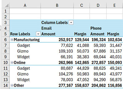
Figure 3 shows the same PivotTable after the macro has run.

2. Fix a spill range limitation

Spill ranges are part of dynamic arrays. They have been covered in many recent articles. Currently, the format doesn’t spill with the values. We can use a macro to fix this limitation.

In Figure 4, the formula in cell B2 has spilled down and across, but the format hasn’t.

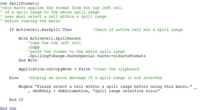
The macro in Figure 5 will format the spill range based on the format of the top-left cell of the spill range. That cell needs to have the required format applied before the macro is run.

Note: This solution is not dynamic. If the spill range is expanded, the macro needs to be rerun.

This macro checks if the active cell is in a spill range. If it isn’t, a message box is used to display an error message.

The ActiveCell.SpillParent command refers to the top-left cell in the spill range. This cell is copied and only its format is pasted to the rest of the spill range.

Figure 6 shows the report after the macro has run.

The macro works on one spill range at a time. If you select a range containing more than one spill range, it will only work on the first spill range.

This macro is especially useful for spill ranges that return dates that must be formatted to display correctly.

3. Insert a hyperlinked file index sheet in seconds

Most Excel files have several sheets. In general, the more complex the file, the more sheets it contains. When a file has a lot of sheets, it is a good idea to include an index sheet with hyperlinks to allow the user to easily navigate to each of the sheets.

Again, creating an index sheet with hyperlinks can be a manual and time-consuming process.

This macro is longer and more complex than the other two. It creates a new sheet called “_INDEX_” when it is first run. It is inserted to the left of the existing sheets. When the macro is run again, it must check to see if that sheet already exists. If the sheet exists, the macro asks the user to confirm that they want to overwrite the existing entries before it continues.

The macro creates two hyperlinked lists of sheet names. One list is in alphabetic order, to make it easier to find a sheet if you know the name. The other list displays in the same order as they appear in the file.

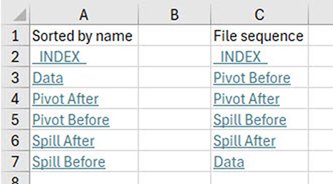
Figure 7 shows an example of the index sheet.

Excel has a shortcut to return after following a hyperlink. Press the F5 function key, and then press Enter.

Macros offer many opportunities to reduce manual processes and speed up frequent tasks.

The companion video and Excel files (Before and After) will go into more detail to demonstrate these techniques.