Excel tips: how to use the index-match combination

Excel has a number of conditional calculation functions. These require ranges that need to be examined or used. Sometimes you need the ability to include a flexible range. The easiest way to include a flexible range is to use an INDEXMATCH combination.

INDEX-MATCH is typically used to extract a single value from a two-dimensional range, but it can also return a range from a two-dimensional range.

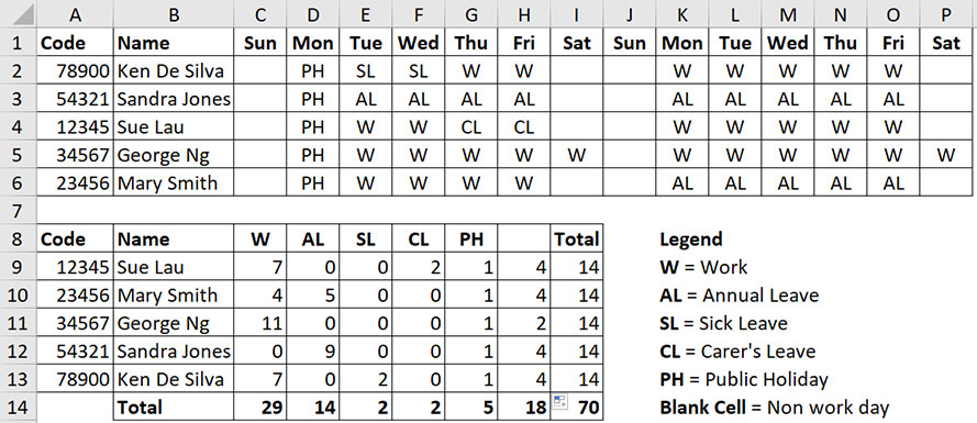
In Figure 01, we have a table of staff with their roster at the top (rows 1 to 6). A summary report (rows 8 to 14) that we need to populate is below. 

The summary list is in a different sequence to the roster above. The names in the top section are sorted by surname, and the summary list is sorted by code.

We need to populate the summary table, which counts how many times the various codes are used in the fortnight.

The COUNTIFS function allows you to count entries based on multiple criteria. In this example, we only need to count a single range per person. If the sequence of staff was the same in the top roster and the summary below, then we could use the following formula in cell C9:

=COUNTIFS($C2:$P2,C$8)

This counts the number of times W (the entry in cell C8) appears in the range C2:P2. Note: COUNTIFS is not case sensitive.

The summary sequence is different to the roster sequence, so we need a flexible way to identify the correct range to count. With the above formula, if the sequence changed, then the table at the bottom may not be accurate.

Creating a flexible range

We can use the INDEX-MATCH combination to conditionally select the correct range to count based on the codes in column A. The following formula will work in cell C9:

=COUNTIFS(INDEX($C$2:$P$6,MATCH($A9,$A$2:$A$6,0),0),C$8)

The range $C2:$P2 from the earlier formula has been replaced with an INDEX-MATCH combination:

INDEX($C$2:$P$6,MATCH($A9,$A$2:$A$6,0),0) 

The INDEX-MATCH combination is often used as an alternative to VLOOKUP. (Note: there is a new function on the way called XLOOKUP, which will replace VLOOKUP. XLOOKUP removes many of VLOOKUP’s limitations and problems.)

The typical INDEX-MATCH formula extracts a single value. In this case, because we have used 0 as the last argument (the INDEX column number argument), the INDEX function will return the whole row within the table, instead of a single cell.

The first argument of the INDEX is the range to extract from. This is the table of entries we need to count. It excludes the headings.

The second argument in the INDEX function is the row number within the range to extract. The MATCH function provides that number by finding the employee code within the entries in the range A2:A6.

When using this technique, you must use a unique code to lookup.

The MATCH function returns a number that represents where a value is within a range:

MATCH($A9,$A$2:$A$6,0)

The first argument of the MATCH is the value to look for, in this case the employee code.

The second argument is the range to look in. Because the MATCH function is returning the row number, its range’s row numbers must line up exactly with the row numbers in the range in the INDEX function. In this case, rows 2 to 6 are being looked up by the MATCH, and those rows match the rows in the INDEX range.

The third argument in the MATCH is the type of lookup required. We need to perform an exact MATCH as we are looking for a specific code. An exact MATCH is selected by entering 0. That completes the MATCH function, which specifi es the row number to extract. In cell C9, the MATCH will return a 3, as the code 12345 is the third code in the range A2:A6.

The third argument of the INDEX function is the column number. As mentioned earlier, we have used 0. This instructs Excel to return the whole row from the range. In the case of the formula in cell C9, the range returned by the INDEX will be C4:P4 for Sue Lau.

In cell C9, this is the range the COUNTIFS function will use to count the occurrences of W. As you copy this formula across it will count the other codes AL, SL, etc.

Handling blanks

In the summary report, we needed to calculate how many cells were empty (column H in the summary report). Cell H8 looks empty, but it contains an unusual formula that works with the COUNTIFS function to count empty cells. The formula in cell H8 is:

=""

Two quotation marks combined refer to a blank/empty cell.

Note: there isn’t a space between the two quotation marks. The COUNTIFS uses that reference to count blank/empty cells.

Dates and days

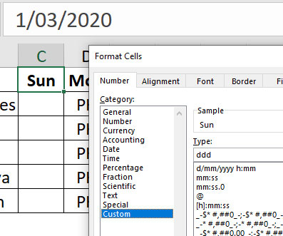
Cell C1 displays Sun, but it contains a date, as you can see in Figure 02. Cell C1 has a custom number format applied, which displays the abbreviated day of the week name. The format used is ddd as per Figure 03. If you wanted the full day name, you would use dddd. 

 

A shortcut to open the Format Cells dialog is Ctrl + 1. Use the 1 on the keyboard, not on the numeric keypad. This shortcut will format anything you have selected in Excel.

The companion video and Excel file will go into more detail to demonstrate these techniques.

Neale Blackwood CPA runs A4 Accounting, providing Excel training, webinars and consulting services to organisations around Australia. Questions can be sent to [email protected]