Loading component...
At a glance
He recently “opened the vault” on those early articles and began to review the information and add newer and easier solutions or built-in functions, plus videos to help users work through the information, which was often written in response to readers’ questions.
This reprised article references Blackwood’s Excel articles from October to December 2002.
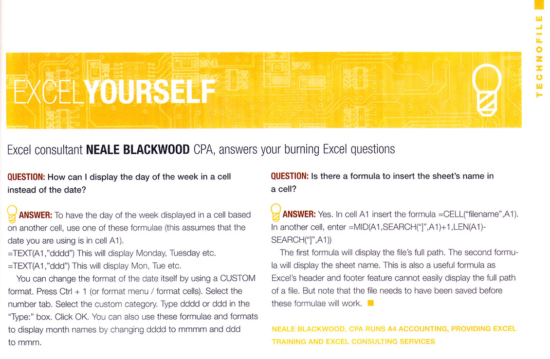
Here is the first Excel Yourself article (yes, I have kept every article I have written).
Just a reminder, this was before Excel 2003 had been released. We were using Excel 97, Excel 2000 and Excel 2002 (also known as Excel XP); yes, years before Facebook, Twitter and YouTube. If you are in your 20s then you were probably in primary school when this was first published.
As you can see, space was at a premium and we didn’t use any screenshots – it was all done with instructions.
One advantage with the latest versions of Excel is the FORMULATEXT function. This function displays the formula from another cell. I have used it in the companion file so you can see the result in the cell and the formula in the cell next to it.
Here are the four questions I covered between October and December 2002:
1. How can I display the day of the week in a cell instead of the date?
This depends on whether you want to display the day of the week instead of the date, or if you want to convert a date into its day of the week.
To have the date display as the day of the week, you can use a Custom Number Format. This is at the bottom of the Number tab of the Format Cells dialog – see Figure 2.
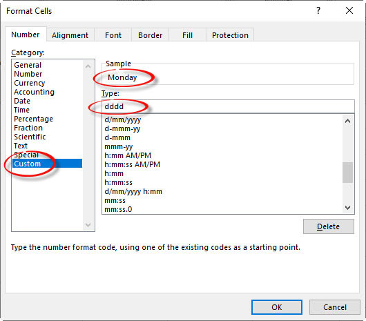
The format codes to use are ddd or dddd.
You enter the code in the Type section. The Sample section shows what the format will look like using the currently selected cell.
ddd displays the three character abbreviation.
dddd displays the full day name.
I included a bonus tip that mmm and mmmm did the same for month names.
Now you can even use mmmmm (that’s five ms) and that will display the first letter of the month. This is commonly used for the bottom axis for month names on dashboard charts where space is at a premium.
I also included a tip on opening the Format Cells dialog using a keyboard shortcut Ctrl + 1. This tip allows you to format anything in Excel, not just cells. Make sure you use the 1 on the keyboard, not the 1 on the numeric keypad.
If you want to use the day of the week in a formula in another cell, you can use the TEXT function. Assuming the date is in cell A1, then this formula displays the full day name. See Figure 3.
=TEXT(A1,"dddd")

2. Is there a formula to insert the sheet’s name in a cell?
I split the answer between two formulas. You can create a single formula to do this, but it is extremely long. In this case it is simpler to split it up. Sometimes in Excel it is better to have two shorter formulas than one long one. Note, the file must have been saved for these formulas to work.
First formula
=CELL("filename",A1)
This formula can be in cell A1 even though it refers to A1 because the CELL function is an information function, not a calculation function. This formula displays the full path of the file with the sheet name on the end. Always refer to a cell in the second argument of the CELL function otherwise you can get incorrect results.
Second formula
=RIGHT(A1,LEN(A1)-SEARCH("]",A1))
Assuming the first formula is in cell A1, then the above formula extracts everything after the ], which is where the sheet name is displayed. The SEARCH function returns a number representing the character position of the value being searched for within another text string.
You can see both formulas in Figure 4.

Single formula
If you are happy to use a long formula, here is the single formula that extracts the sheet name:
=RIGHT(CELL("filename",A1),LEN(CELL("filename",A1))-SEARCH("]",CELL("filename",A1)))
Extracting the sheet name can allow you to automate reports. Let’s say a report on a sheet summarises department costs using a department code and SUMIFS functions. Instead of manually entering the department code, you could use one of the above formulas to extract the department code from the sheet name. Then changing the sheet name will automatically update the report. If you copy the sheet and change its name, you have a new report for a new department. It works like a report template. Sheet names are useful because Excel won’t allow you to duplicate sheet names.
3. Can Excel extract unique entries from a column?
The answer involved the Advanced Filter in the Data ribbon, but there are a couple of other ways to do this.
Advanced Filter
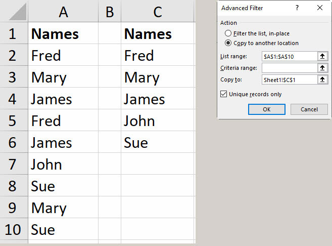
Click inside the column A list and click the Data ribbon, then click the Advanced option in the Sort & Filter section. Make the changes as per the dialog in Figure 5 and click OK.
Remove Duplicates
Copy the list to another location. With a cell selected in the pasted list, click the Data ribbon and click the Remove Duplicates icon. Click OK, and it’s done.
PivotTable
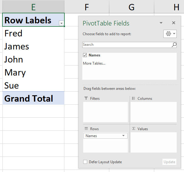
A quicker way is to use a PivotTable and drag the column name to the Rows section of the PivotTable – job done.
Click inside the column and press Alt n v (this opens the Create PivotTable dialog). Tick the Existing Worksheet (you could also leave the default to create in a new sheet) and select a cell in the current sheet and click OK. Drag the field to the Names section – job done. See Figure 6.
4. Is there a way to select all the cells that have a formula?
This involves the Go To dialog. These days there is a quicker way to select all the formulas in a range in one step.
One reason to select all the formulas is to format them with a consistent colour. Using colours consistently is best practice, for example, colour for input cells.
Nowadays (from Excel 2013 onwards) you can even use a conditional format to apply colour to formulas automatically.
Select formula cells
If you have a single cell selected when you use this technique it will analyse the whole sheet. If you have range selected, it will only analyse the range.
On the Home ribbon click the Find & Select icon (far right) and choose Formulas. Job done. When they are all selected you could change their format.
Formatting formula cells automatically
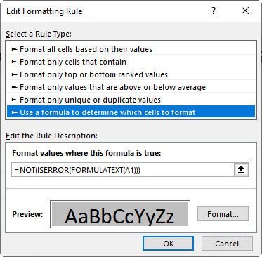
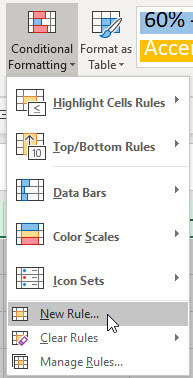
This works in Excel 2013 on later versions. Press Ctrl + A to select the whole sheet. Click the Conditional Formatting icon on the Home ribbon. Select New Rule from the dropdown – see Figure 7.
Select the last option in the top section (“use a formula …”) and enter the following formula in the box below:
=NOT(ISERROR(FORMULATEXT(A1)))
The formula in the box must return TRUE for the formula to be applied.
The FORMULATEXT function returns an error if a cell doesn’t have a formula. The ISERROR will return FALSE if the cell has a formula and TRUE it if doesn’t. This is the opposite of what we need to apply the conditional format. The NOT function corrects that. The NOT function changes TRUE to FALSE and FALSE to TRUE. The final formula returns TRUE for formula cells.
Click the Format button and select a fill colour – I have used grey in Figure 8 – then click OK.
