Loading component...
At a glance
My December 2020 article on Excel used slicers and a formatted table. Range names work well with input cells, allowing the user to make selections that automatically update the chart.
Dynamic charts enable the user to modify inputs and immediately see the results in reports and dashboards. This technique uses range names to enable the interaction.
Date data
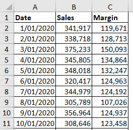
We’ll be using a sequential date data table to drive the chart. The data extract is shown in Figure 1.

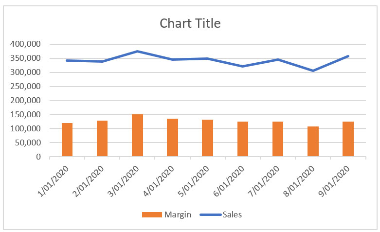
This has daily sales and margin values from 1 January 2020 to 10 January 2020. We will plot the sales on a line chart and display the margin as a column chart.
We will create the chart normally by selecting a small range as the chart data source, and then we will amend certain entries to make the chart dynamic.
Select the range A1 to C10. Then, click on the Insert ribbon tab, click the column chart icon drop-down and choose the first chart, a clustered column chart.

Right-click the Sales series on the chart and choose Change Series Chart Type. Select Line from the Chart Type drop-down for Sales and click OK. Figure 2 has the amended chart.
Range names
We will create three range names, one each for the dates, sales and the margins. These range names will use INDEX functions to define their ranges and make them dynamic. We will then edit the chart’s source data to incorporate the range names.

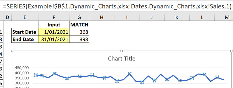
The range names will expand and contract based on the two date input cells, F2 and F3 – see Figure 3.
The cells G2 and G3 are helper cells that will make the final formulas shorter. They contain MATCH functions. The formula in cell G2 has been copied down and is
=MATCH(F2,A:A,0)
The MATCH function returns a number that represents the position of an item within a range. The first argument in the function is the item to search for, the second is the range to search in. The zero at the end means you require an exact match. This means if the item is not in the range, the #N/A error is displayed. Note: the latest version of Excel has a new function called XMATCH, which has a few more search options. It is currently only available in the subscription version of Excel.
Cell G2 displays 368 because the date 1/1/2021 is in row 368 of the list. By using the whole column as the range to search in you are, in effect, returning the row number of the item being searched for. The date 31/1/2021 is on row 398.
Creating the range names
Click the Formulas ribbon tab and click the Define Name icon from the Defined Names section. In the dialog that opens, enter Dates as the name, and use the following formula in the Refers to box. Click OK to create the name. Note: the sheet name is Example.
=INDEX(Example!$A:$A,Example!$G$2)
:INDEX(Example!$A:$A,Example!$G$3)
The INDEX function allows you to select a cell from a range (first argument), based on a row number (second argument) and a column number (third argument) from within that range. In the above example, we can omit the column number (third argument) and just use the row number (second argument), because the range is a single column. By using an INDEX function on either side of the colon, we create a fully dynamic range. The first INDEX defines the start cell, and the second INDEX defines the end cell. The above formula currently refers to the range A368:A398 based on row numbers that are in cells G2 and G3.
Use the Define Name icon to create two more range names. See below for names and formulas. You can copy the formula from the first name and modify it for the other two names.
Sales
=INDEX(Example!$B:$B,Example!$G$2)
:INDEX(Example!$B:$B,Example!$G$3)
Margin
=INDEX(Example!$C:$C,
Example!$G$2):INDEX
(Example!$C:$C,Example!$G$3)
There is a trick to editing a formula in the New Name dialog and other Excel dialogs. To use the arrow keys to move around, press the F2 function key, which changes the mode to edit. If you don’t press F2, then using the arrow keys will insert cell references from the sheet.I will demonstrate this in the companion video to this article, which you can watch by clicking the button at top right of this page.
You could also use the OFFSET function to create these range formulas. I avoid the OFFSET function if there is an alternative, because it is volatile, meaning it calculates each time Excel calculates, whether it needs to or not. Most functions, like the INDEX, only re-calculate when their range changes. The more volatile functions you use, the slower larger models become.
Amending the chart data source

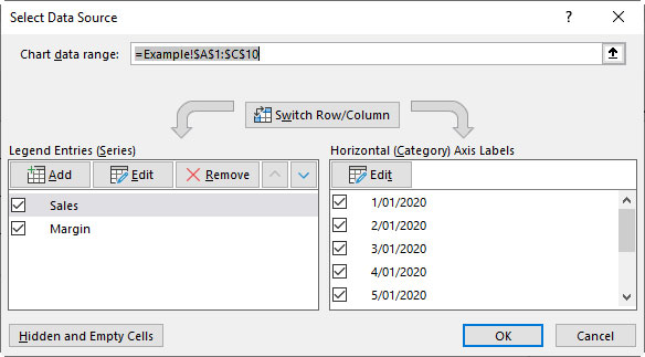
Right-click the chart and click Select Data – see Figure 4.
Click the Edit button on the right side, in the Horizontal (Category) Axis Labels section.
Change the formula to
=Examples!Dates
Click OK.
Click Sales on the left of the dialog, then click the Edit button above and then change the Series values formula to
=Example!Sales
Click OK.
Click Margin on the left of the dialog, click the Edit button above and then change the Series values formula to
=Example!Margin
Click OK, then OK again. Job done.
Changing the dates in cells F2 or F3 will now update the chart.
Note: If you go back and edit the Sales or Margins entries again, you will find the file name in front of the range name, not the sheet name. I am not sure why, but the sheet name is retained for the Dates range name.
Series function

If you click on the Sales line chart and examine the Formula Bar, you will see that the range names are listed in a SERIES function – see Figure 5.
If you are plotting a single data series, you can modify this SERIES function in the Formula Bar to make the range name modifications. The 1 on the end of the SERIES function means it is the first data series. There appears to be a bug when editing the SERIES function except for the first data series. I will demonstrate the bug in the companion video to this article.
Dynamic ranges based on data
This example created dynamic range names based on inputs. Depending on your requirements, you could create automated dynamic ranges based on existing data, for example, the first date and last date in a data set. When the data set is updated, the dates could automatically change, and the dynamic range updates. You can use the MIN and MAX functions to find the earliest and the latest dates in a list, respectively.
The companion video and Excel files (blank and complete) will go into more detail to demonstrate these techniques.
Neale Blackwood CPA runs A4 Accounting, providing Excel training, webinars and consulting. Questions can be sent to [email protected]

