Loading component...
At a glance

I have three Excel state report files in a folder. There are other files in the folder as well. I want to import all three report files and convert the report layout into a data layout. I can then use the data layout with pivot tables to report on the combined data.
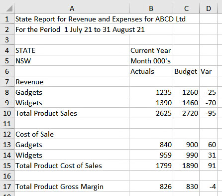
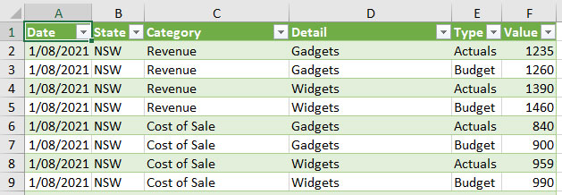
The top section of the report layout can be seen in Figure 1. The goal is to create a data layout as shown in Figure 2.

This is something that used to be achieved with custom written macros. With Power Query, this process can be automated via the user interface with one straightforward formula.
This is a scalable technique. If we add another state report file to the folder, it will automatically be imported the next time the data is refreshed.
The other files in the folder will need to be ignored. A naming convention allows you to filter out unnecessary files. If other files have similar names, you may need to rename them or remove them from the folder.
Versions
I will be using the subscription version of Excel for this example. Older versions may have slightly different button labels. Power Query is constantly being updated, so changes are inevitable.
Power Query is on the left-hand side of the Data ribbon. It has its own ribbon in earlier Excel versions.
Procedures
1. In the Data ribbon, click the Get Data drop-down and choose From File, then choose From Folder.
2. Navigate to the XL_Data folder. Select the folder and click Open. All files, in any subfolders, will also be imported.
3. An interim window opens showing all files in the folders and subfolders. Click the Combine drop-down and choose Combine and Transform Data.
4. Another interim window opens. This lists the sheets in the file. It defaults to using the first file to base this list on. Click the Sample File dropdown and select one of the files with a name that starts with Report_. Click the Report sheet underneath, under Parameters. The sheet structure will appear on the right of dialog. Click OK.
5. The Power Query Editor window opens. In the table that displays, use the filter icon on the first column to select Text Filter, then Begins With. Type in Report_ and click OK. This will exclude unwanted files. I have used the underscore character in the file naming convention. Use a Text filter and Ends With, and enter .xlsx. This ensures only Excel files will be included.
6. The Power Query steps so far are listed on the right of the screen. These steps are repeated each time the data is refreshed. Note: When working in the Power Query window, there is no Undo or Redo icon. You can undo steps by deleting them using the red cross on the left of the step, but there is no dedicated Undo option.
7. Right-click the first column header and choose Replace Values. In the top box, enter .xlsx and leave the bottom box empty. Click OK. This removes the Excel file extension from the file name.
8. Right-click the first column header and choose Split Column, then choose By Delimiter. In the top drop-down, make sure --Custom-- is selected and the underscore character is shown below it. Click OK. This splits the Source.Name column across three columns – see Figure 3. A delimiter is a character (or characters) that separates parts of a text entry or code. In our case, the underscore character separates parts of the file name that we can use as column entries.

9. Right-click the first column and remove it.
10. Double the column headers to rename the first five columns in the following sequence across the table: Date, State, Detail, Actuals and Budget. The columns on the right that weren’t renamed can be deleted.
11. On the Home ribbon, click the Remove Row drop-down and choose Remove Top Rows. Enter 5 in the dialog that opens and click OK.
12. Use the filter icon on the Detail column and untick the null option at the top of the list. In Power Query (null means a blank, or no entry). Note: Whenever you refer to null, it is always entered in lowercase. Power Query is case sensitive, so be careful when typing entries. The null option is always listed at the top of the filter list. By filtering the table, you are reducing the number of rows that will be loaded, which can speed up refresh times.
13. We now need to work on the report structure to capture the categories as a separate column. There are descriptive headings above the value lines. We need to capture them in a separate column.
14. In the Add Column ribbon tab, click the Custom Column option. Change the name to Category. In the formula box, enter the following formula. Note that the = sign is always in the Formula box.
If [Actuals] = null and [Budget] = null then [Detail] else null
You can double-click the column names on the right of the dialog to enter the names surrounded by square brackets. This is case sensitive, so be careful. If you have an error, check both the spelling and the case.
15. Right-click the Category column and choose Fill, then choose Down. This captures the categories on the correct rows.
16. Filter the Actuals column and remove the null entries.
17. There are headings in the Actuals column. To remove them, click the ABC123 icon on the left of the column header and choose Whole Number. This generates errors for all text entries.
18. Right-click the Actuals column and choose Remove Errors.
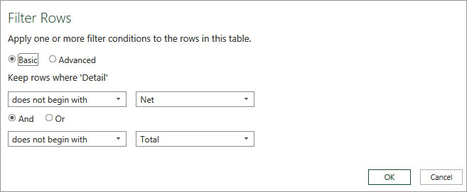
19. There are total rows in the data. We could leave them there, but it will be cleaner if we remove them. Filter the Detail column and use Text filters. Use two Does Not Begin With criteria options, separated by the And option. The first is Net and the second is Total. Click OK – see Figure 4

20. We are now ready to convert the report into a data layout.
21. Move the Category column to the left of the Detail column by dragging its header across.
22. Select the first four columns by holding the Ctrl key down and clicking each column. Then right-click one of the selected column headings and choose Unpivot other columns.
23. Change the Attribute column name to Type. Change the Value column data type to Whole Number.
24. Click the Home ribbon and the Close and Load option on the left to import the data from all three files.
The filter rules you use are important, and need to be robust. They may require some trial and error to perfect.
I used the null option a couple of times to remove rows. If the report had used an empty (null) cell for a zero value (for example, there were no stock adjustments for the month), then using null would not have worked correctly.
You should also check your Power Query output against the original data to make sure nothing has been missed.
The companion video and Excel files will go into more detail to demonstrate these techniques.
Neale Blackwood CPA runs A4 Accounting, providing Excel training, webinars and consulting services. Questions can be sent to [email protected]

