Excel Tips: Import data into Excel from a PDF file

PDF files are used for invoices, statements, orders and so much more. They can contain useful information that may be used for analysis, reporting and reconciliations. 

In the past, capturing that information has been a challenge. Often third-party applications have been used to convert PDF files into tables for Excel.

While they may do a good job, these third-party products may not offer the data-cleansing features of Power Query, which is part of Excel. 

Power Query can also automate the PDF importation process, whereas using third-party software tends to require manual processes. Third-party software may also come with a fee.  

The example that follows imports a publicly available PDF file created by the Australian Taxation Office (ATO). It contains the monthly tax tables for the 2024–25 Australian tax year. You can find the PDF on this page.

Not all PDFs are created equal. Some are easy to import, whereas others offer a few challenges. Due to the variability in PDF file quality and structure, trial and error may be required to achieve the desired output.

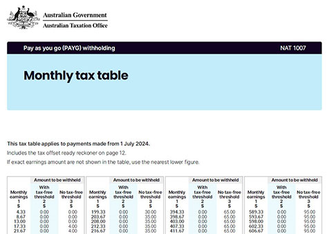
The layout of the document is shown in Figure 1.

There are four separate tables across each page and there are 12 pages. 

To import the PDF file, follow these steps.

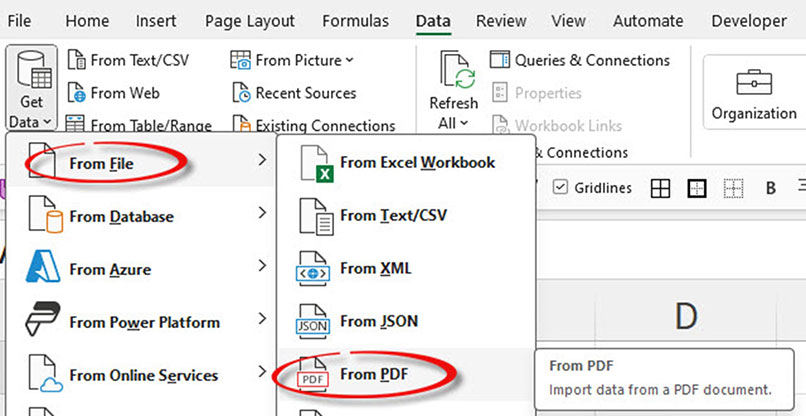
1. In the Data ribbon tab, click the Get Data icon drop-down and choose From File and then From PDF. See Figure 2.

2. Navigate to the location of the PDF file, select it and click Import.

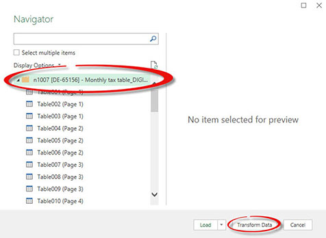
3. In the Navigator window, click the folder icon for the file on the left and then click the Transform Data button at the bottom right – see Figure 3.

4. In the Power Query Editor window in the third column there are two Kinds listed. Page and Table. See Figure 4.

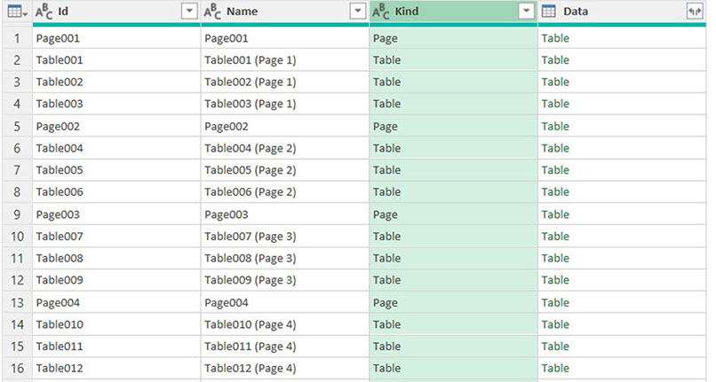
Filter the Kind column by Table. In general, always filter by Table in the first attempt to import a PDF. If that doesn’t work, try again and filter by Page. You must filter by one of them because they each contain the same data.

5. Click the small double arrow icon in the top right of the Data column header.

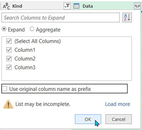
6. In the dialog that opens (Figure 5), untick the option Use original column name as prefix. Click OK. This brings in all the data from all the tables.

7. The first three columns (Id, Name and Kind) are no longer required and can be deleted, leaving the three columns we want to import – see Figure 6.

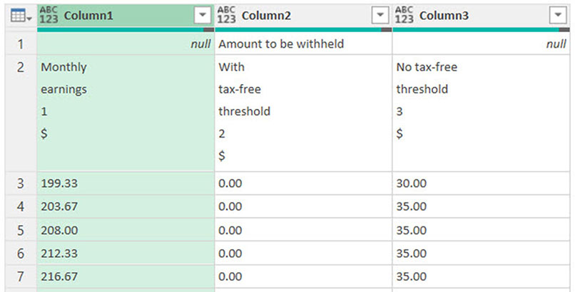
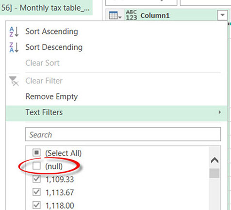
8. Each separate table in the PDF has a table heading. Above each heading is a row that has the words Amount to be withheld in Column2. These extra rows can be removed by filtering out the null entries in Column1. In Power Query, null means a blank or empty cell. The null option is always listed at the top of the filter options – see Figure 7.

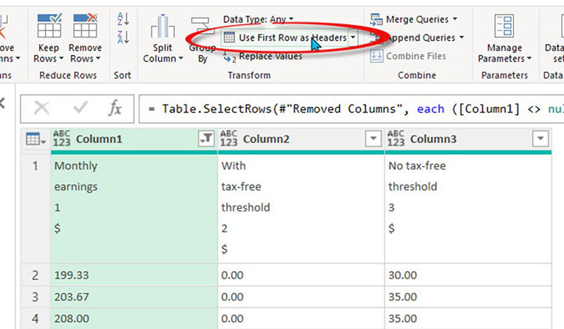
9. The first row of the data now has the table headings. On the Home ribbon, click the Use First Row as Headers icon to capture the column names. This is called Promoting the Headers – see Figure 8.

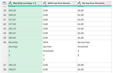
10. The other table headers in the data are visible as you scroll down – see Figure 9.

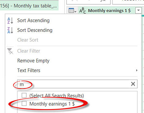
11. To remove the other headers, click the filter icon for the first column (Monthly earnings 1 $) and in the Search box type m. This will limit the entries and show just the header text. Untick the text Monthly earnings 1 $ and click OK – see Figure 10.

12. Next, change the data type for all columns to Currency. On the left of each column header click the ABC icon and select Currency.

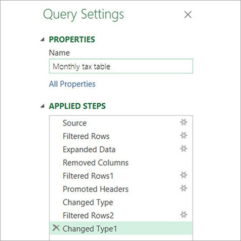
13. All the steps performed have been captured on the right of screen. The default name uses the file name. You can change that to Monthly tax table – see Figure 11.

14. Click the Close & Load icon on the far left of the Home ribbon. That creates a table on a sheet called Monthly tax table – see Figure 12.

15. Notice that there are seven errors (far right of Figure 12). The blue 7 errors is a clickable link that opens the Power Query window. It creates a separate query that lists the error lines as a separate table and lists their row numbers. See Figure 13.

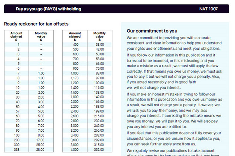
16. The row numbers are all at the end of the table. Reviewing the PDF file, we can see that the last page has a different layout and different tables. See Figure 14.

17. It is common for the end of a PDF to have a different structure. With the Power Query Window open,  click the Monthly tax table query.  

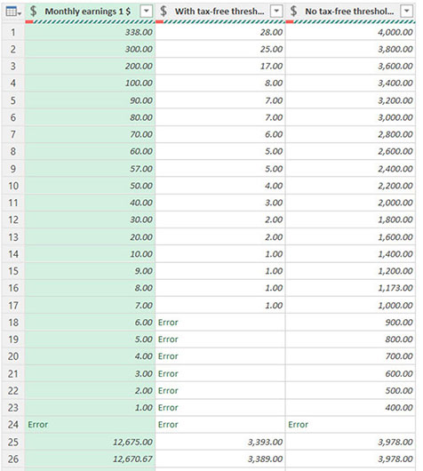
18. To quickly see the entries at the bottom of the list, click the Transform ribbon tab and click the Reverse Rows option. This is quicker than scrolling. The result is shown in Figure 15.

19. One row (24) has errors in all columns. Right click the first column and choose Remove Errors.

20. In the remaining unwanted rows at the top, the values in the third column are all greater than the values in the first column. That rule doesn’t apply to the tax table rows to be retained. A new column can be added to enable a filter to remove the unwanted rows.

21. Click the Add Column ribbon tab and click the Custom Column icon. In the dialog that opens, click in the Custom column formula section. Double click the No tax-free threshold column on the right of the dialog. Type > and then double click the Monthly Earnings column on the right – see Figure 16. Click OK.

22. A  new column is inserted that displays FALSE for the rows we want to remove. Apply a filter to this column to remove the FALSE rows. You can delete the new custom column after you have filtered the table.

23. The final step is to return the table to the original sequence. Click the Transform ribbon tab and click the Reverse Rows icon. On the Home ribbon, click the Close & Load button to complete the import process.  

This import was a one-off, as tax rates don’t often change. If you were importing a monthly statement from a supplier, you could re-run the query next month to import the latest PDF statement. 

Each PDF file is different and the steps you take to fix problems will vary. Power Query has many built-in processes that can help convert badly laid-out data into well laid-out data. 

Find more INTHEBLACK Power Query articles here.

CPA Australia offers a range of Excel courses, which you can find here.