Loading component...
At a glance
I shared an automated loan schedule in my July 2020 article. Recently, someone asked if I could create a loan schedule with an interest-free period, using formulas.
I tried and failed. I got close, but couldn’t get the loan to finish on zero until I thought of Goal Seek. Goal Seek is a simple trial-and-error tool. You specify a goal cell and a goal value, then specify a cell to change to reach that goal. The change cell must affect the goal cell. Goal Seek tries different values and hones in on the solution. It doesn’t always solve it.
Goal Seek is a manual process, but it should solve our problem.
Worked example
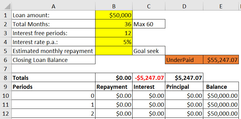
This solution includes a few different techniques you can use for other situations. Figure 1 has the sheet structure we will work with.

The yellow cells are for input. Cell B5 will be populated by Goal Seek. Note: the repayment amount is entered as a negative. We need a monthly repayment value that will clear the loan in the number of months entered in cell B2.
Cell E6 extracts the balance from the last period of the loan from the schedule beneath it. This cell should be zero. If the value isn’t zero, these two cells will have an orange fill colour. I have used a conditional format on both cells with a tolerance of 1. The conditional formatting settings for these will be shared in the companion video.
The formula in cell D6 displays text based on the value in cell E6. This formula is
=IF(ABS(E6)<=1,"",IF(E6<0,"Over Paid","Under Paid"))
The loan schedule starting in row 8 uses the monthly repayment value from cell B5.
Goal Seek will be used to find the repayment that returns a zero (or near zero value) balance.
Goal SEEK steps
1. Select cell E6. This will capture the Set cell: for the next step.
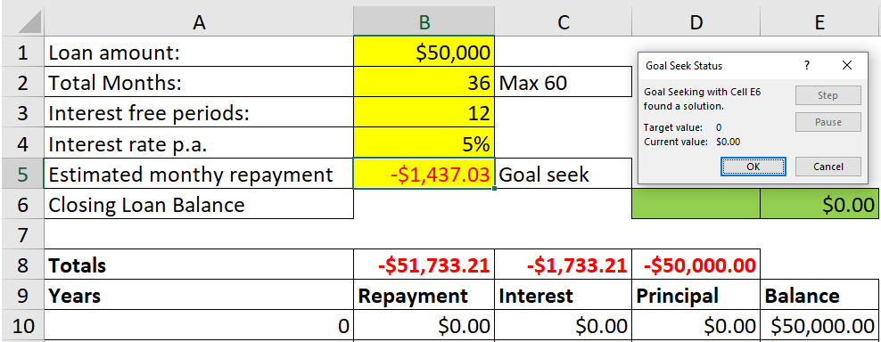
2. Click the Data ribbon tab and click the What-If Analysis icon drop-down (far right) and select Goal Seek. See Figure 2 for the dialog that opens and the entries required.

3. Enter 0 in the To value: box and B5 in the By changing cell: box and click OK.
4. Another dialog displays informing you if the goal has been achieved – see Figure 3. Clicking Cancel will clear the amount from B5. Clicking OK will accept the amount. Click Undo to remove the amount if needed.

In all, about seven clicks or entries are needed to calculate the repayment using Goal Seek. Goal Seek doesn’t retain previous settings, so you must re-enter them each time. A recorded macro could automate Goal Seek and we could run it off a button.
Developer tab
Working with macros is easier if you display the Developer ribbon tab. To do that, rightclick the ribbon and choose Customize the Ribbon. On the right-hand side listing, tick the Developer box and click OK.
Macro warning: when you run a macro, it clears the Undo list. This means you can’t undo what the macro did or anything you did before you ran the macro. Save the file before running a macro, so you can close and not save if something goes wrong.
If you’re saving a file with a new macro, make sure you choose the macro-enabled file type (.xlsm) or the binary file type (.xlsb). The normal Excel file type (.xlsx) doesn’t save macros.

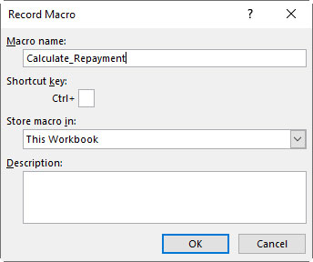
Click the Developer tab and click the Record Macro icon in the top left. Figure 4 shows the dialog that opens.
In the Macro name: box, enter Calculate_Repayment and make sure the Store macro in: box has This Workbook. If it doesn’t, use the drop-down to select it. Click OK. Note: macro names can’t contain spaces.
Repeat steps 1 to 4 above. Once Goal Seek is finished, stop the macro recording. Click the Developer ribbon tab and click Stop Recording (where the Record Macro icon was previously).
Now that we’ve a recorded macro, we can assign it to a shape to make it easy to run from the sheet.
Click the Insert tab and click the Shapes drop-down. I will use a rounded corner rectangle. Draw the shape on the sheet and enter the text Calculate Repayment. If you start typing after drawing the shape, it will automatically insert the text.
Right-click the shape and choose Assign Macro. In the dialog that opens, make sure This Workbook is selected in the drop-down, select the Calculate_Repayment macro and click OK.
Clicking the shape will now run the macro.
Try changing some of the loan input values. This will cause cells D6 and E6 to change colour. Click the shape to update the repayment and cells D6 and E6 should return to green.
Editing the macro
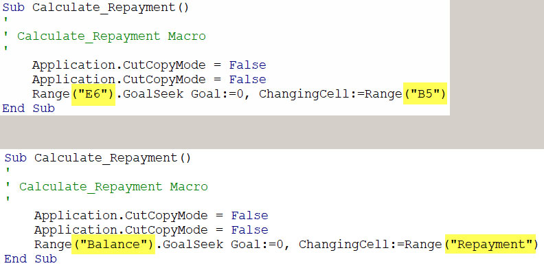
When you record a macro, Excel hard-keys the cell references into the code. This means if the structure of the sheet changes (rows or columns are inserted or deleted), the references in the macro may no longer be valid. To avoid that, we can use two range names for the two cells we reference, then edit the recorded macro to use those range names.
Click in cell B5 and click in the Name Box. This is the box on the left of the Formula Bar, above the column letters. It usually has the current cell reference in it. Type Repayment in the Name Box and press Enter.
Click in cell E6 and click in the Name Box. Type Balance and press Enter. Note: range names can’t contain spaces either.
To edit the recorded macro, click the Developer ribbon tab and click the Macros icon. Select the Calculate_Repayment name and then click the Edit button on the right.
Change the E6 reference to Balance and the B5 reference to Repayment. Make sure you keep all the quotation marks – see Figure 5.

By using Goal Seek and a macro, we were able to return a value that is difficult to return with a formula. In the companion video, I will demonstrate a further enhancement where we can automate the Goal Seek macro to run whenever one of the loan input cells is updated.
The companion video and Excel files (Loan and Loan Macro) will go into more detail to demonstrate these techniques.
Neale Blackwood CPA runs A4 Accounting, providing Excel training, webinars and consulting services. Questions can be sent to [email protected]

