Loading component...
At a glance

This article is based on a question from a CPA Australia member who wanted to convert an existing budget structure into a forecast structure. The example relates to wages, but could be applied to any situation where you have costs that start and stop.
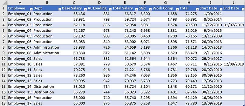
In Figure 1, columns A to H were used to create the initial wages budget. I have added and populated the Start Date and End Date columns to enable forecasting.

The wages assumptions used in Figure 1 are shown in column M in Figure 2, which also includes a fortnightly breakdown of the wages based on the table from Figure 1. In future, this forecast structure could be used as the budget.
Creating the forecast
The formatted table in Figure 1 has been named WagesForecast via the Design ribbon tab that is displayed when the table is selected. Formatted tables were covered in the August 2018 edition of INTHEBLACK.
A date in the End Date column determines the last fortnight that the employee will be paid. A date in the Start Date column will determine the first fortnightly payment.
It is important to note that the formulas used may not provide an accurate wage calculation for the first fortnightly payment of a new employee or the last fortnight payment of a terminating employee. Since this is a forecast, that level of accuracy is considered acceptable.
If we use the names built into the formatted table (called structured references), the formulas become very long. Copying the formulas across columns can also be problematic. This is because of the way in which the structured references are handled by Excel.
To get around these issues we can use range names to define the columns that we need to use from the table. They will have the advantages of the formatted table names in that they will automatically expand as the table expands, but they won’t have the drawbacks mentioned above.
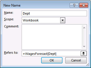
We need to create four names to use in our formulas. We first select the column of data that we want to name. The quick way to do that is to click a cell in that column and press Ctrl + Space. Using the Department column as an example, we will select the range B2:B18. Press Ctrl + Alt + F3 (or click the Formulas tab and click the Define Name icon) to open the New Name dialog.

In the Name box enter Dept and click OK (see Figure 3). Note the structured reference used in the “Refers to” box.
We need to repeat the above process for three more names by selecting ranges in the other columns. The other names we need to create are Total (H2:H18), Start (I2:I18) and End (J2:J18). Once created, the names can be used in formulas.
As structured references have been used in the “Refers to” box, these four names automatically expand as new rows are added to the table.
The formula for cell P2 in Figure 2 is:
=SUMPRODUCT(Total*(Start<=O2)*((End>=O2)+(End="")))/26
The divide by 26" converts the annual figure into a fortnight amount.
The SUMPRODUCT function is Excel’s most flexible function. In this case, it is performing a calculation similar to a SUMIFS function, but it is doing something that the SUMIFS can’t handle. You would require two SUMIFS functions to achieve what the single SUMPRODUCT function has done.
As the End Date column contains a blank if the employee is still employed, we need to check that in the conditions that we set. We need to check for either a date that is greater than or equal to pay date in column O, or a blank cell. The SUMIFS function only sums when all conditions are met; it doesn’t cope when you want one of two conditions met. The SUMPRODUCT function allows you to create an OR criteria, where we identify if one of two or more conditions is met.
Formula explanation
The SUMPRODUCT function sums up the results of product calculations. In mathematics the product of two numbers is achieved by multiplying them together. SUMPRODUCT multiplies numbers together, then adds up the result.
The SUMPRODUCT function allows you to compare a range of cells to a single cell. In doing so it creates a listing of TRUE and FALSE results, one for each cell comparison. In Excel, TRUE = 1 and FALSE = 0.
The Total at the start of the function refers to the Total column in Figure 1 – it has all the values that we will add up.
(Start<=O2)
This is a condition that confirms that the Start Date is earlier (less than) or equal to the fortnight payroll date in column O. Only the last two dates in the start column in the table (new employees) are after the first fortnight date in cell O2.
If the date is less than or equal to the fortnight date TRUE is returned, otherwise FALSE is returned.
((End>=O2)+(End=""))
This is the calculation that the SUMIFS function can’t handle. It checks that the End date is after (greater than) or equal to the date in column O or that the cell is blank. Using "" refers to a blank cell. A blank cell means the employee will be there for the full year; i.e. no end date.
The important thing about this check is that the two checks are mutually exclusive. If one is TRUE, then the other has to be FALSE. They could both be FALSE, but they can’t both be TRUE. The + sign between the two conditions means the results could be:
FALSE (0) + FALSE (0) = FALSE (0)
TRUE (1) + FALSE (0) = TRUE (1)
FALSE (0) + TRUE (1) = TRUE (1)

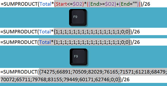
Remember, TRUE and TRUE is not possible. The * symbols between the conditions convert the TRUE and FALSE results into ones and zeros respectively. This can be seen in Figure 4. When you select part of a formula and press the F9 function key, Excel displays the results.
The ones and zeros are multiplied by the values in the Total column to arrive at the values for the fortnight. The bottom of Figure 4 show two zeros. These relate to the two new employees who won’t be paid in the first fortnight.
We can amend this formula to only add up a particular department. The formula in cell Q2 is:
=SUMPRODUCT(Total*(Dept=Q$1)*(Start<=$O2)*((End>=$O2)+(End="")))/26
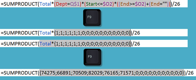
This has the added condition (Dept=Q$1), which confirms the department in the table matches the department in cell Q1 (Production). This formula can be copied across and down for the other departments.

You can see the different results with the added department condition in Figure 5.
The SUMPRODUCT function allows you to perform calculations with advanced conditions. In the companion video, I will also demonstrate the SUMIFS solutions for the above formulas. The companion file has examples of all the calculations.
The companion video and Excel file will go into more detail to demonstrate these techniques.
Questions can be sent to [email protected].

